

8.14 Collocation Method for Obtaining Normal Modes …
351
If certain function of x is equal to a certain function of t, then both will be equal
to a constant. Choosing p
2 as the constant
Y (x) = p
2
L
0
f (x, ξ)ρ A(ξ )Y (ξ )dξ
(8.182)
and
¨
q + p
2 q = 0
(8.183)
Equation (8.183) is equivalent to the differential equation [Eq. (8.82)]. The
solution will consist of infinite sets of eigenvalues and the corresponding set of
eigenfunctions Y (x).
In the method of collocation, we reduce the problem to a finite number of equations
of motion.
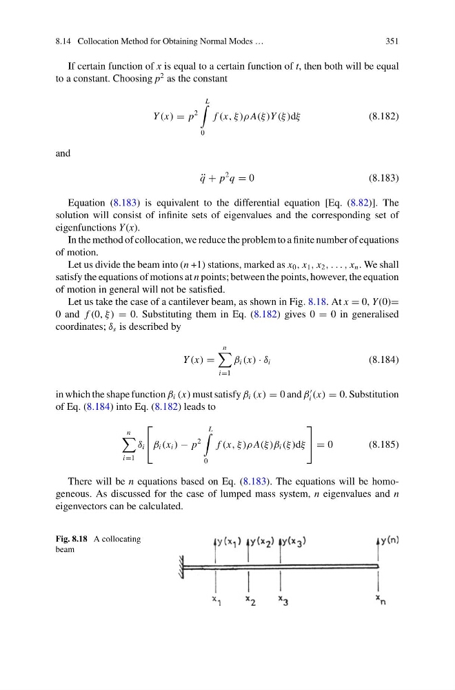
Let us divide the beam into (n +1) stations, marked as x 0 , x 1 , x 2 , . . . , x n . We shall
satisfy the equations of motions at n points; between the points, however, the equation
of motion in general will not be satisfied.
Let us take the case of a cantilever beam, as shown in Fig. 8.18. At x = 0, Y (0)=
0 and f (0, ξ) = 0. Substituting them in Eq. (8.182) gives 0 = 0 in generalised
coordinates; δ s is described by
Y (x) =
n
i=1
β i (x) · δ i
(8.184)
in which the shape function β i (x) must satisfy β i (x) = 0 and β
i (x) = 0. Substitution
of Eq. (8.184) into Eq. (8.182) leads to
n
i=1
δ i
⎡
⎣ β i (x i ) − p
2
L
0
f (x, ξ)ρ A(ξ )β i (ξ )dξ
⎤
⎦ = 0
(8.185)
There will be n equations based on Eq. (8.183). The equations will be homogeneous. As discussed for the case of lumped mass system, n eigenvalues and n
eigenvectors can be calculated.
Fig. 8.18 A collocating
beam
351
If certain function of x is equal to a certain function of t, then both will be equal
to a constant. Choosing p
2 as the constant
Y (x) = p
2
L
0
f (x, ξ)ρ A(ξ )Y (ξ )dξ
(8.182)
and
¨
q + p
2 q = 0
(8.183)
Equation (8.183) is equivalent to the differential equation [Eq. (8.82)]. The
solution will consist of infinite sets of eigenvalues and the corresponding set of
eigenfunctions Y (x).
In the method of collocation, we reduce the problem to a finite number of equations
of motion.
Let us divide the beam into (n +1) stations, marked as x 0 , x 1 , x 2 , . . . , x n . We shall
satisfy the equations of motions at n points; between the points, however, the equation
of motion in general will not be satisfied.
Let us take the case of a cantilever beam, as shown in Fig. 8.18. At x = 0, Y (0)=
0 and f (0, ξ) = 0. Substituting them in Eq. (8.182) gives 0 = 0 in generalised
coordinates; δ s is described by
Y (x) =
n
i=1
β i (x) · δ i
(8.184)
in which the shape function β i (x) must satisfy β i (x) = 0 and β
i (x) = 0. Substitution
of Eq. (8.184) into Eq. (8.182) leads to
n
i=1
δ i
⎡
⎣ β i (x i ) − p
2
L
0
f (x, ξ)ρ A(ξ )β i (ξ )dξ
⎤
⎦ = 0
(8.185)
There will be n equations based on Eq. (8.183). The equations will be homogeneous. As discussed for the case of lumped mass system, n eigenvalues and n
eigenvectors can be calculated.
Fig. 8.18 A collocating
beam