

7.12 Frequency Domain Analysis of Direct Frequency Response Method
301
= F
(r )
0 e
i(ωt+α r )
or,
F r = F
(r )
0 [cos(ωt + α r ) + i sin(ωt + α r )]
(7.109)
Now,
{F(t)} =
F
∗
e
iωt
(7.110)
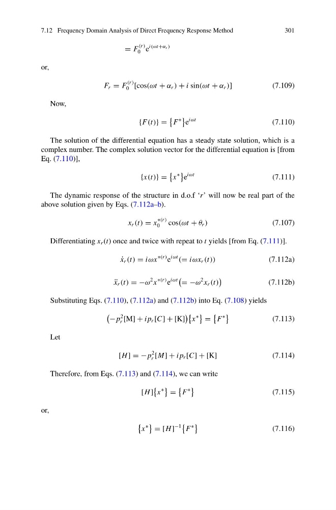
The solution of the differential equation has a steady state solution, which is a
complex number. The complex solution vector for the differential equation is [from
Eq. (7.110)],
{x(t)} =
x
∗
e
iωt
(7.111)
The dynamic response of the structure in d.o.f ‘r’ will now be real part of the
above solution given by Eqs. (7.112a–b).
x r (t) = x
∗(r )
0
cos(ωt + θ r )
(7.107)
Differentiating x r (t) once and twice with repeat to t yields [from Eq. (7.111)].
˙
x r (t) = iωx
∗(r ) e
iωt
(= iωx r (t))
(7.112a)
¨
x r (t) = −ω
2 x
∗(r ) e
iωt
= −ω
2 x r (t)
(7.112b)
Substituting Eqs. (7.110), (7.112a) and (7.112b) into Eq. (7.108) yields
− p
2
r [M] + i p r [C] + [K]
x
∗
=
F
∗
(7.113)
Let
[H ] = −p
2
r [M] + i p r [C] + [K]
(7.114)
Therefore, from Eqs. (7.113) and (7.114), we can write
[H ]
x
∗
=
F
∗
(7.115)
or,
x
∗
= [H ]
−1
F
∗
(7.116)
301
= F
(r )
0 e
i(ωt+α r )
or,
F r = F
(r )
0 [cos(ωt + α r ) + i sin(ωt + α r )]
(7.109)
Now,
{F(t)} =
F
∗
e
iωt
(7.110)
The solution of the differential equation has a steady state solution, which is a
complex number. The complex solution vector for the differential equation is [from
Eq. (7.110)],
{x(t)} =
x
∗
e
iωt
(7.111)
The dynamic response of the structure in d.o.f ‘r’ will now be real part of the
above solution given by Eqs. (7.112a–b).
x r (t) = x
∗(r )
0
cos(ωt + θ r )
(7.107)
Differentiating x r (t) once and twice with repeat to t yields [from Eq. (7.111)].
˙
x r (t) = iωx
∗(r ) e
iωt
(= iωx r (t))
(7.112a)
¨
x r (t) = −ω
2 x
∗(r ) e
iωt
= −ω
2 x r (t)
(7.112b)
Substituting Eqs. (7.110), (7.112a) and (7.112b) into Eq. (7.108) yields
− p
2
r [M] + i p r [C] + [K]
x
∗
=
F
∗
(7.113)
Let
[H ] = −p
2
r [M] + i p r [C] + [K]
(7.114)
Therefore, from Eqs. (7.113) and (7.114), we can write
[H ]
x
∗
=
F
∗
(7.115)
or,
x
∗
= [H ]
−1
F
∗
(7.116)