

7.4 Response of MDF Systems Under the Action of Transient Forces
269
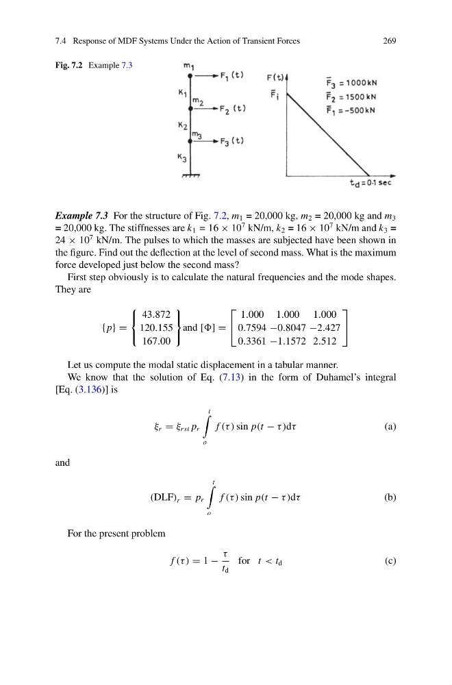
Fig. 7.2 Example 7.3
Example 7.3 For the structure of Fig. 7.2, m 1 = 20,000 kg, m 2 = 20,000 kg and m 3
= 20,000 kg. The stiffnesses are k 1 = 16 × 10
7 kN/m, k 2 = 16 × 10
7 kN/m and k 3 =
24 × 10
7 kN/m. The pulses to which the masses are subjected have been shown in
the figure. Find out the deflection at the level of second mass. What is the maximum
force developed just below the second mass?
First step obviously is to calculate the natural frequencies and the mode shapes.
They are
{ p} =
⎧
⎨
⎩
43.872
120.155
167.00
⎫
⎬
⎭
and [] =
⎡
⎣
1.000 1.000 1.000
0.7594 −0.8047 −2.427
0.3361 −1.1572 2.512
⎤
⎦
Let us compute the modal static displacement in a tabular manner.
We know that the solution of Eq. (7.13) in the form of Duhamel’s integral
[Eq. (3.136)] is
ξ r = ξ rst p r
t
o
f (τ ) sin p(t − τ )dτ
(a)
and
(DLF) r = p r
t
o
f (τ ) sin p(t − τ )dτ
(b)
For the present problem
f (τ ) = 1 −
τ
t d
for t < t d
(c)
269
Fig. 7.2 Example 7.3
Example 7.3 For the structure of Fig. 7.2, m 1 = 20,000 kg, m 2 = 20,000 kg and m 3
= 20,000 kg. The stiffnesses are k 1 = 16 × 10
7 kN/m, k 2 = 16 × 10
7 kN/m and k 3 =
24 × 10
7 kN/m. The pulses to which the masses are subjected have been shown in
the figure. Find out the deflection at the level of second mass. What is the maximum
force developed just below the second mass?
First step obviously is to calculate the natural frequencies and the mode shapes.
They are
{ p} =
⎧
⎨
⎩
43.872
120.155
167.00
⎫
⎬
⎭
and [] =
⎡
⎣
1.000 1.000 1.000
0.7594 −0.8047 −2.427
0.3361 −1.1572 2.512
⎤
⎦
Let us compute the modal static displacement in a tabular manner.
We know that the solution of Eq. (7.13) in the form of Duhamel’s integral
[Eq. (3.136)] is
ξ r = ξ rst p r
t
o
f (τ ) sin p(t − τ )dτ
(a)
and
(DLF) r = p r
t
o
f (τ ) sin p(t − τ )dτ
(b)
For the present problem
f (τ ) = 1 −
τ
t d
for t < t d
(c)