

7.3 Mode-Acceleration Method for the Determination …
267
Therefore
x 1 (t) =
1
48 × 10 7 × 8P cos ωt
+
ω
2
1924.733
(1.0)P cos ωt
20,000 × 1.6896 × (1924.733 − ω 2 )
⎤
⎥
⎥
⎦ N = 1
+
ω
2
14437.20
(1.0)P cos ωt
20,000 × 2.9867 × (14437.20 − ω 2 )
⎤
⎥
⎥
⎥
⎥
⎥
⎥
⎥
⎦
N = 2
+
ω
2
27,889
(1.0)P cos ωt
20,000 × 13.2 × (27,889 − ω 2 )
⎤
⎥
⎥
⎥
⎥
⎥
⎥
⎥
⎥
⎥
⎥
⎥
⎦
N = 3
(c)
Let
C o =
x 1 (t)
P cos ωt
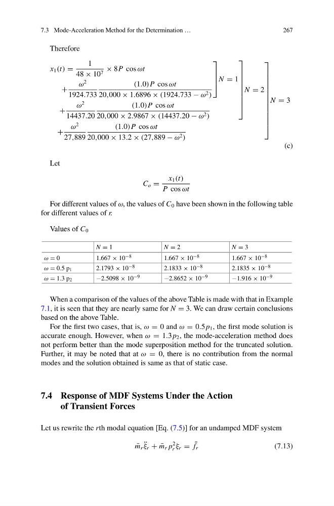
For different values of ω, the values of C 0 have been shown in the following table
for different values of r.
Values of C 0
N = 1
N = 2
N = 3
ω = 0
1.667 × 10 −8
1.667 × 10 −8
1.667 × 10 −8
ω = 0.5 p 1
2.1793 × 10 −8
2.1833 × 10 −8
2.1835 × 10 −8
ω = 1.3 p 2
−2.5098 × 10 −9
−2.8652 × 10 −9
−1.916 × 10 −9
When a comparison of the values of the above Table is made with that in Example
7.1, it is seen that they are nearly same for N = 3. We can draw certain conclusions
based on the above Table.
For the first two cases, that is, ω = 0 and ω = 0.5 p 1 , the first mode solution is
accurate enough. However, when ω = 1.3 p 2 , the mode-acceleration method does
not perform better than the mode superposition method for the truncated solution.
Further, it may be noted that at ω = 0, there is no contribution from the normal
modes and the solution obtained is same as that of static case.
7.4 Response of MDF Systems Under the Action
of Transient Forces
Let us rewrite the rth modal equation [Eq. (7.5)] for an undamped MDF system
¯
m r ¨
ξ r + ¯
m r p
2
r ξ r = ¯
f r
(7.13)
267
Therefore
x 1 (t) =
1
48 × 10 7 × 8P cos ωt
+
ω
2
1924.733
(1.0)P cos ωt
20,000 × 1.6896 × (1924.733 − ω 2 )
⎤
⎥
⎥
⎦ N = 1
+
ω
2
14437.20
(1.0)P cos ωt
20,000 × 2.9867 × (14437.20 − ω 2 )
⎤
⎥
⎥
⎥
⎥
⎥
⎥
⎥
⎦
N = 2
+
ω
2
27,889
(1.0)P cos ωt
20,000 × 13.2 × (27,889 − ω 2 )
⎤
⎥
⎥
⎥
⎥
⎥
⎥
⎥
⎥
⎥
⎥
⎥
⎦
N = 3
(c)
Let
C o =
x 1 (t)
P cos ωt
For different values of ω, the values of C 0 have been shown in the following table
for different values of r.
Values of C 0
N = 1
N = 2
N = 3
ω = 0
1.667 × 10 −8
1.667 × 10 −8
1.667 × 10 −8
ω = 0.5 p 1
2.1793 × 10 −8
2.1833 × 10 −8
2.1835 × 10 −8
ω = 1.3 p 2
−2.5098 × 10 −9
−2.8652 × 10 −9
−1.916 × 10 −9
When a comparison of the values of the above Table is made with that in Example
7.1, it is seen that they are nearly same for N = 3. We can draw certain conclusions
based on the above Table.
For the first two cases, that is, ω = 0 and ω = 0.5 p 1 , the first mode solution is
accurate enough. However, when ω = 1.3 p 2 , the mode-acceleration method does
not perform better than the mode superposition method for the truncated solution.
Further, it may be noted that at ω = 0, there is no contribution from the normal
modes and the solution obtained is same as that of static case.
7.4 Response of MDF Systems Under the Action
of Transient Forces
Let us rewrite the rth modal equation [Eq. (7.5)] for an undamped MDF system
¯
m r ¨
ξ r + ¯
m r p
2
r ξ r = ¯
f r
(7.13)