

232
6 Free Vibration of Multiple Degrees of Freedom System
The equations of motion of the system are given by
F = − [M] { ¨
ξ } − [K ] {ξ } + {F} = {0}
(6.111)
[M] and [K ] will be diagonal matrices only for the normal modes. As in this procedure, the calculations are based on the assumption of mode shapes, it is quite likely
that Eq. (6.111) will be in coupled form. However, a good choice of assumed mode
shapes will make off-diagonal terms relatively small. For free vibration of the system,
the following solution is assumed
{ξ } = {A } sin pt
(6.112)
Substituting the solution assumed in Eq. (6.112) into Eq. (6.111), the equation of
motion becomes
([K ] − p
2
[M]) {A } = {0}
(6.113)
Solution of eigenvalue problem given by Eq. (6.108) will yield the eigenvalues.
Example 6.13 For the problem given in Example 6.9, determine the first two natural
frequencies by Rayleigh–Ritz method, assuming the first two mode shapes.
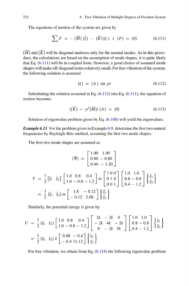
The first two mode shapes are assumed as
[] =
⎡
⎣
1.00 1.00
0.80 − 0.80
0.40 − 1.20
⎤
⎦
T =
1
2
˙
ξ 1 ˙
ξ 2
1.0 0.8 0.4
1.0 − 0.8 − 1.2
m
⎡
⎣
1 0 0
0 1 0
0 0 1
⎤
⎦
⎡
⎣
1.0 1.0
0.8 − 0.8
0.4 − 1.2
⎤
⎦
˙
ξ 1
˙
ξ 2
=
1
2
[ ˙
ξ 1 ˙
ξ 2 ] m
1.8 − 0.12
− 0.12 3.08
˙
ξ 1
˙
ξ 2
Similarly, the potential energy is given by
U =
1
2
{ξ 1 ξ 2 }
1.0 0.8 0.4
1.0 − 0.8 − 1.2
⎡
⎣
2k − 2k 0
− 2k 4k − 2k
0 − 2k 5k
⎤
⎦
⎡
⎣
1.0 1.0
0.8 − 0.8
0.4 − 1.2
⎤
⎦
ξ 1
ξ 2
=
1
2
{ξ 1 ξ 2 } k
0.88 − 0.4
− 0.4 11.12
ξ 1
ξ 2
For free vibration, we obtain from Eq. (6.118) the following eigenvalue problem
6 Free Vibration of Multiple Degrees of Freedom System
The equations of motion of the system are given by
F = − [M] { ¨
ξ } − [K ] {ξ } + {F} = {0}
(6.111)
[M] and [K ] will be diagonal matrices only for the normal modes. As in this procedure, the calculations are based on the assumption of mode shapes, it is quite likely
that Eq. (6.111) will be in coupled form. However, a good choice of assumed mode
shapes will make off-diagonal terms relatively small. For free vibration of the system,
the following solution is assumed
{ξ } = {A } sin pt
(6.112)
Substituting the solution assumed in Eq. (6.112) into Eq. (6.111), the equation of
motion becomes
([K ] − p
2
[M]) {A } = {0}
(6.113)
Solution of eigenvalue problem given by Eq. (6.108) will yield the eigenvalues.
Example 6.13 For the problem given in Example 6.9, determine the first two natural
frequencies by Rayleigh–Ritz method, assuming the first two mode shapes.
The first two mode shapes are assumed as
[] =
⎡
⎣
1.00 1.00
0.80 − 0.80
0.40 − 1.20
⎤
⎦
T =
1
2
˙
ξ 1 ˙
ξ 2
1.0 0.8 0.4
1.0 − 0.8 − 1.2
m
⎡
⎣
1 0 0
0 1 0
0 0 1
⎤
⎦
⎡
⎣
1.0 1.0
0.8 − 0.8
0.4 − 1.2
⎤
⎦
˙
ξ 1
˙
ξ 2
=
1
2
[ ˙
ξ 1 ˙
ξ 2 ] m
1.8 − 0.12
− 0.12 3.08
˙
ξ 1
˙
ξ 2
Similarly, the potential energy is given by
U =
1
2
{ξ 1 ξ 2 }
1.0 0.8 0.4
1.0 − 0.8 − 1.2
⎡
⎣
2k − 2k 0
− 2k 4k − 2k
0 − 2k 5k
⎤
⎦
⎡
⎣
1.0 1.0
0.8 − 0.8
0.4 − 1.2
⎤
⎦
ξ 1
ξ 2
=
1
2
{ξ 1 ξ 2 } k
0.88 − 0.4
− 0.4 11.12
ξ 1
ξ 2
For free vibration, we obtain from Eq. (6.118) the following eigenvalue problem