

204
6 Free Vibration of Multiple Degrees of Freedom System
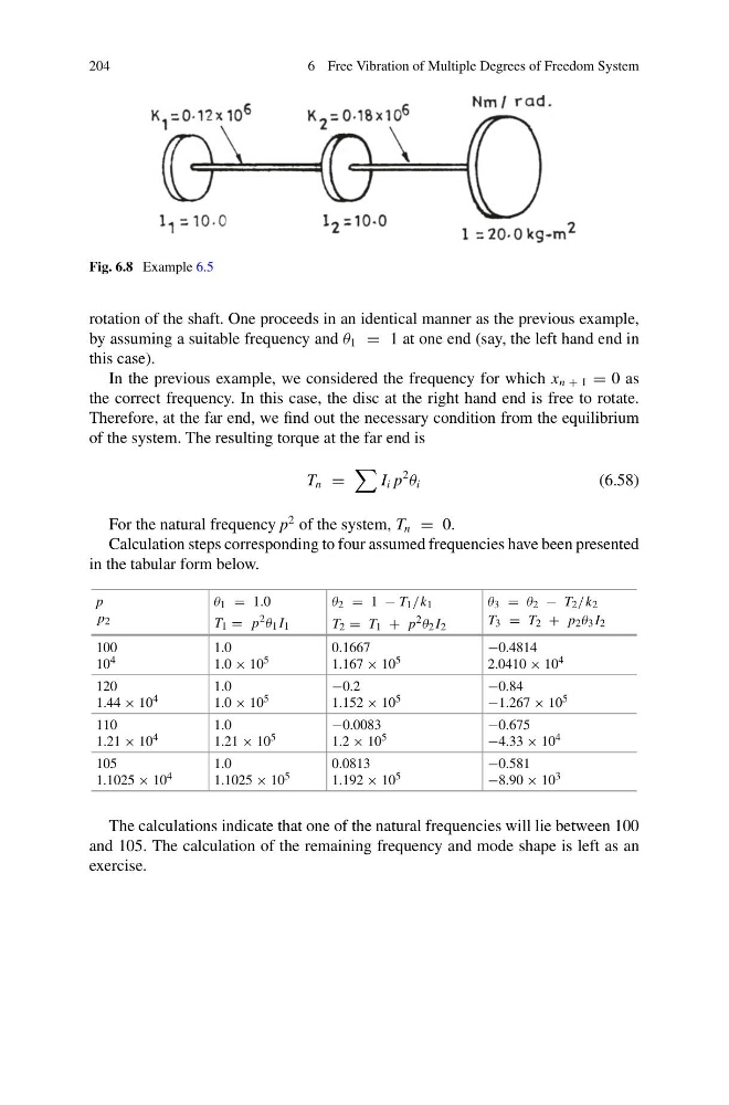
Fig. 6.8 Example 6.5
rotation of the shaft. One proceeds in an identical manner as the previous example,
by assuming a suitable frequency and θ 1 = 1 at one end (say, the left hand end in
this case).
In the previous example, we considered the frequency for which x n + 1 = 0 as
the correct frequency. In this case, the disc at the right hand end is free to rotate.
Therefore, at the far end, we find out the necessary condition from the equilibrium
of the system. The resulting torque at the far end is
T n =
I i p
2
θ i
(6.58)
For the natural frequency p
2 of the system, T n = 0.
Calculation steps corresponding to four assumed frequencies have been presented
in the tabular form below.
p
p 2
θ 1 = 1.0
T 1 = p 2 θ 1 I 1
θ 2 = 1 − T 1 /k 1
T 2 = T 1 + p 2 θ 2 I 2
θ 3 = θ 2 − T 2 /k 2
T 3 = T 2 + p 2 θ 3 I 2
100
10 4
1.0
1.0 × 10 5
0.1667
1.167 × 10 5
−0.4814
2.0410 × 10 4
120
1.44 × 10 4
1.0
1.0 × 10 5
−0.2
1.152 × 10 5
−0.84
−1.267 × 10 5
110
1.21 × 10 4
1.0
1.21 × 10 5
−0.0083
1.2 × 10 5
−0.675
−4.33 × 10 4
105
1.1025 × 10 4
1.0
1.1025 × 10 5
0.0813
1.192 × 10 5
−0.581
−8.90 × 10 3
The calculations indicate that one of the natural frequencies will lie between 100
and 105. The calculation of the remaining frequency and mode shape is left as an
exercise.
6 Free Vibration of Multiple Degrees of Freedom System
Fig. 6.8 Example 6.5
rotation of the shaft. One proceeds in an identical manner as the previous example,
by assuming a suitable frequency and θ 1 = 1 at one end (say, the left hand end in
this case).
In the previous example, we considered the frequency for which x n + 1 = 0 as
the correct frequency. In this case, the disc at the right hand end is free to rotate.
Therefore, at the far end, we find out the necessary condition from the equilibrium
of the system. The resulting torque at the far end is
T n =
I i p
2
θ i
(6.58)
For the natural frequency p
2 of the system, T n = 0.
Calculation steps corresponding to four assumed frequencies have been presented
in the tabular form below.
p
p 2
θ 1 = 1.0
T 1 = p 2 θ 1 I 1
θ 2 = 1 − T 1 /k 1
T 2 = T 1 + p 2 θ 2 I 2
θ 3 = θ 2 − T 2 /k 2
T 3 = T 2 + p 2 θ 3 I 2
100
10 4
1.0
1.0 × 10 5
0.1667
1.167 × 10 5
−0.4814
2.0410 × 10 4
120
1.44 × 10 4
1.0
1.0 × 10 5
−0.2
1.152 × 10 5
−0.84
−1.267 × 10 5
110
1.21 × 10 4
1.0
1.21 × 10 5
−0.0083
1.2 × 10 5
−0.675
−4.33 × 10 4
105
1.1025 × 10 4
1.0
1.1025 × 10 5
0.0813
1.192 × 10 5
−0.581
−8.90 × 10 3
The calculations indicate that one of the natural frequencies will lie between 100
and 105. The calculation of the remaining frequency and mode shape is left as an
exercise.