

6.9 Holzer Method
203
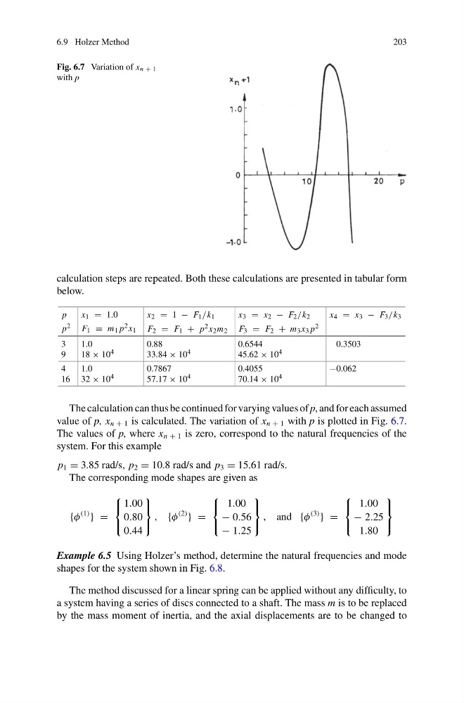
Fig. 6.7 Variation of x n + 1
with p
calculation steps are repeated. Both these calculations are presented in tabular form
below.
p
p 2
x 1 = 1.0
F 1 = m 1 p 2 x 1
x 2 = 1 − F 1 /k 1
F 2 = F 1 + p 2 x 2 m 2
x 3 = x 2 − F 2 /k 2
F 3 = F 2 + m 3 x 3 p 2
x 4 = x 3 − F 3 /k 3
3
9
1.0
18 × 10 4
0.88
33.84 × 10 4
0.6544
45.62 × 10 4
0.3503
4
16
1.0
32 × 10 4
0.7867
57.17 × 10 4
0.4055
70.14 × 10 4
−0.062
The calculation can thus be continued for varying values of p, and for each assumed
value of p, x n + 1 is calculated. The variation of x n + 1 with p is plotted in Fig. 6.7.
The values of p, where x n + 1 is zero, correspond to the natural frequencies of the
system. For this example
p 1 = 3.85 rad/s, p 2 = 10.8 rad/s and p 3 = 15.61 rad/s.
The corresponding mode shapes are given as
{φ
(1)
} =
⎧
⎨
⎩
1.00
0.80
0.44
⎫
⎬
⎭
, {φ
(2)
} =
⎧
⎨
⎩
1.00
− 0.56
− 1.25
⎫
⎬
⎭
, and {φ
(3)
} =
⎧
⎨
⎩
1.00
− 2.25
1.80
⎫
⎬
⎭
Example 6.5 Using Holzer’s method, determine the natural frequencies and mode
shapes for the system shown in Fig. 6.8.
The method discussed for a linear spring can be applied without any difficulty, to
a system having a series of discs connected to a shaft. The mass m is to be replaced
by the mass moment of inertia, and the axial displacements are to be changed to
203
Fig. 6.7 Variation of x n + 1
with p
calculation steps are repeated. Both these calculations are presented in tabular form
below.
p
p 2
x 1 = 1.0
F 1 = m 1 p 2 x 1
x 2 = 1 − F 1 /k 1
F 2 = F 1 + p 2 x 2 m 2
x 3 = x 2 − F 2 /k 2
F 3 = F 2 + m 3 x 3 p 2
x 4 = x 3 − F 3 /k 3
3
9
1.0
18 × 10 4
0.88
33.84 × 10 4
0.6544
45.62 × 10 4
0.3503
4
16
1.0
32 × 10 4
0.7867
57.17 × 10 4
0.4055
70.14 × 10 4
−0.062
The calculation can thus be continued for varying values of p, and for each assumed
value of p, x n + 1 is calculated. The variation of x n + 1 with p is plotted in Fig. 6.7.
The values of p, where x n + 1 is zero, correspond to the natural frequencies of the
system. For this example
p 1 = 3.85 rad/s, p 2 = 10.8 rad/s and p 3 = 15.61 rad/s.
The corresponding mode shapes are given as
{φ
(1)
} =
⎧
⎨
⎩
1.00
0.80
0.44
⎫
⎬
⎭
, {φ
(2)
} =
⎧
⎨
⎩
1.00
− 0.56
− 1.25
⎫
⎬
⎭
, and {φ
(3)
} =
⎧
⎨
⎩
1.00
− 2.25
1.80
⎫
⎬
⎭
Example 6.5 Using Holzer’s method, determine the natural frequencies and mode
shapes for the system shown in Fig. 6.8.
The method discussed for a linear spring can be applied without any difficulty, to
a system having a series of discs connected to a shaft. The mass m is to be replaced
by the mass moment of inertia, and the axial displacements are to be changed to