

5.7 Coordinate Coupling
169
connected to two ends of the bar. To describe the motion of the system, it has two
degrees of freedom—the vertical translation y and rotation θ as shown. The origin
is considered at the point of static equilibrium. For free vibration of the system, the
forces acting on it are shown in Fig. 5.10b.
Equation of motion for the system for vertical motion is
m ¨
y + 2m
¨
y +
L
2
¨
θ
+ k
y −
L
2
θ
+ 2k
y +
L
2
θ
= 0
or,
3m ¨
y + m L ¨
θ + 3ky +
k L
2
θ = 0
(5.35)
Taking moment of the forces about the origin as shown in Fig. 5.10b
2m
¨
y +
L
2
¨
θ
L
2
+ 2k
y +
L
2
θ
L
2
− k
y −
L
2
θ
L
2
= 0
or,
m L ¨
y +
1
2
m L
2 ¨
θ +
k L
2
y +
3
4
k L
2
θ = 0
(5.36)
Writing Eqs. (5.35) and (5.36) in matrix form, we get
3m mL
m L
mL
2
2
¨
y
¨
θ
+
3k
kL
2
kL
2
3
4
k L
2
y
θ
=
0
0
(5.37)
Equation (5.37) indicates the existence of coupling between the independent coordinates. If the mass matrix is non-diagonal, then it is dynamic coupling. If the stiffness matrix is non-diagonal, it is called static coupling. Equation (5.37) reveals both
dynamic and static coupling. Equation (5.1) reveals the static coupling only. Two or
multiple degrees of freedom systems always have coupled equations. The techniques
of uncoupling the equations have been shown in the next chapter.
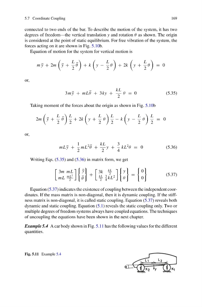
Example 5.4 A car body shown in Fig. 5.11 has the following values for the different
quantities.
Fig. 5.11 Example 5.4
169
connected to two ends of the bar. To describe the motion of the system, it has two
degrees of freedom—the vertical translation y and rotation θ as shown. The origin
is considered at the point of static equilibrium. For free vibration of the system, the
forces acting on it are shown in Fig. 5.10b.
Equation of motion for the system for vertical motion is
m ¨
y + 2m
¨
y +
L
2
¨
θ
+ k
y −
L
2
θ
+ 2k
y +
L
2
θ
= 0
or,
3m ¨
y + m L ¨
θ + 3ky +
k L
2
θ = 0
(5.35)
Taking moment of the forces about the origin as shown in Fig. 5.10b
2m
¨
y +
L
2
¨
θ
L
2
+ 2k
y +
L
2
θ
L
2
− k
y −
L
2
θ
L
2
= 0
or,
m L ¨
y +
1
2
m L
2 ¨
θ +
k L
2
y +
3
4
k L
2
θ = 0
(5.36)
Writing Eqs. (5.35) and (5.36) in matrix form, we get
3m mL
m L
mL
2
2
¨
y
¨
θ
+
3k
kL
2
kL
2
3
4
k L
2
y
θ
=
0
0
(5.37)
Equation (5.37) indicates the existence of coupling between the independent coordinates. If the mass matrix is non-diagonal, then it is dynamic coupling. If the stiffness matrix is non-diagonal, it is called static coupling. Equation (5.37) reveals both
dynamic and static coupling. Equation (5.1) reveals the static coupling only. Two or
multiple degrees of freedom systems always have coupled equations. The techniques
of uncoupling the equations have been shown in the next chapter.
Example 5.4 A car body shown in Fig. 5.11 has the following values for the different
quantities.
Fig. 5.11 Example 5.4