

144
4 Numerical Methods in Structural Dynamics …
A (t) =
1
mp
t
0
F (τ ) cos pτ dτ
(4.33)
B (t) =
1
mp
t
0
F (τ ) sin pτ dτ
(4.34)
Thus, the evaluation of x(t) is primarily numerical integration of A(t) and B(t).
This can be done by various means. Here we adopt Simpson’s rule.
The variation of the displacement with time is of interest. Time is divided into a
number of equal intervals, each of duration τ, and the response at these sequences
of time is to be evaluated. It must be noted that though the time interval is τ, the
response is obtained at 2τ, time intervals, if Simpson’s rule is adopted.
Applying Simpson’s rule, numerical integration of Eq. (4.34) is
A (t) = A (t − 2 ) +
τ
3mp
[F (t − 2 ) cos p (t − 2τ )
+ 4F (t − τ ) cos p (t − τ ) + F (t) cos p t]
(4.35)
A(t − 2τ ) is the value of the integral at time instant (t − 2τ ) obtained by the
summation of the proceeding values.
B(t) of Eq. (4.35) can be numerically integrated in a similar manner.
The procedure is explained with the help of an example.
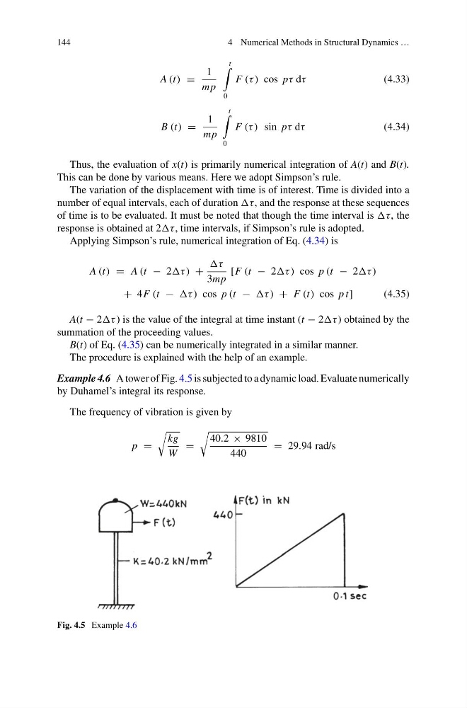
Example 4.6 A tower of Fig. 4.5 is subjected to a dynamic load. Evaluate numerically
by Duhamel’s integral its response.
The frequency of vibration is given by
p =
kg
W
=
40.2 × 9810
440
= 29.94 rad/s
Fig. 4.5 Example 4.6
4 Numerical Methods in Structural Dynamics …
A (t) =
1
mp
t
0
F (τ ) cos pτ dτ
(4.33)
B (t) =
1
mp
t
0
F (τ ) sin pτ dτ
(4.34)
Thus, the evaluation of x(t) is primarily numerical integration of A(t) and B(t).
This can be done by various means. Here we adopt Simpson’s rule.
The variation of the displacement with time is of interest. Time is divided into a
number of equal intervals, each of duration τ, and the response at these sequences
of time is to be evaluated. It must be noted that though the time interval is τ, the
response is obtained at 2τ, time intervals, if Simpson’s rule is adopted.
Applying Simpson’s rule, numerical integration of Eq. (4.34) is
A (t) = A (t − 2 ) +
τ
3mp
[F (t − 2 ) cos p (t − 2τ )
+ 4F (t − τ ) cos p (t − τ ) + F (t) cos p t]
(4.35)
A(t − 2τ ) is the value of the integral at time instant (t − 2τ ) obtained by the
summation of the proceeding values.
B(t) of Eq. (4.35) can be numerically integrated in a similar manner.
The procedure is explained with the help of an example.
Example 4.6 A tower of Fig. 4.5 is subjected to a dynamic load. Evaluate numerically
by Duhamel’s integral its response.
The frequency of vibration is given by
p =
kg
W
=
40.2 × 9810
440
= 29.94 rad/s
Fig. 4.5 Example 4.6