

4.3 Numerical Evaluation of Duhamel’s Integral
143
well for numerical evaluation. If we use this expression as it stands, then the values
of ˙
x and ¨
x and obtained from the previous instants are not required for computing
˙
x and ¨
x at any time instant, and fresh computations for the previous instants are
required at any time instant. The procedure thus demands an impractically large
number of computations [5]. This is explained with the help of an example of a SDF
system, in consistent units m = 2, p = 31.6, x 0 = 0, ˙
x 0 = 0, ,t = 0.02
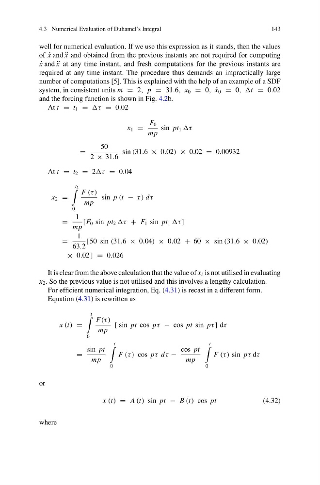
and the forcing function is shown in Fig. 4.2b.
At t = t 1 = τ = 0.02
x 1 =
F 0
mp
sin pt 1 τ
=
50
2 × 31.6
sin (31.6 × 0.02) × 0.02 = 0.00932
At t = t 2 = 2τ = 0.04
x 2 =
t 2
0
F (τ )
mp
sin p (t − τ ) dτ
=
1
mp
[F 0 sin pt 2 τ + F 1 sin pt 1 τ ]
=
1
63.2
[ 50 sin (31.6 × 0.04) × 0.02 + 60 × sin (31.6 × 0.02)
× 0.02 ] = 0.026
It is clear from the above calculation that the value of x i is not utilised in evaluating
x 2 . So the previous value is not utilised and this involves a lengthy calculation.
For efficient numerical integration, Eq. (4.31) is recast in a different form.
Equation (4.31) is rewritten as
x (t) =
t
0
F(τ )
mp
[ sin pt cos pτ − cos pt sin pτ ] dτ
=
sin pt
mp
t
0
F (τ ) cos pτ dτ −
cos pt
mp
t
0
F (τ ) sin pτ dτ
or
x (t) = A (t) sin pt − B (t) cos pt
(4.32)
where
143
well for numerical evaluation. If we use this expression as it stands, then the values
of ˙
x and ¨
x and obtained from the previous instants are not required for computing
˙
x and ¨
x at any time instant, and fresh computations for the previous instants are
required at any time instant. The procedure thus demands an impractically large
number of computations [5]. This is explained with the help of an example of a SDF
system, in consistent units m = 2, p = 31.6, x 0 = 0, ˙
x 0 = 0, ,t = 0.02
and the forcing function is shown in Fig. 4.2b.
At t = t 1 = τ = 0.02
x 1 =
F 0
mp
sin pt 1 τ
=
50
2 × 31.6
sin (31.6 × 0.02) × 0.02 = 0.00932
At t = t 2 = 2τ = 0.04
x 2 =
t 2
0
F (τ )
mp
sin p (t − τ ) dτ
=
1
mp
[F 0 sin pt 2 τ + F 1 sin pt 1 τ ]
=
1
63.2
[ 50 sin (31.6 × 0.04) × 0.02 + 60 × sin (31.6 × 0.02)
× 0.02 ] = 0.026
It is clear from the above calculation that the value of x i is not utilised in evaluating
x 2 . So the previous value is not utilised and this involves a lengthy calculation.
For efficient numerical integration, Eq. (4.31) is recast in a different form.
Equation (4.31) is rewritten as
x (t) =
t
0
F(τ )
mp
[ sin pt cos pτ − cos pt sin pτ ] dτ
=
sin pt
mp
t
0
F (τ ) cos pτ dτ −
cos pt
mp
t
0
F (τ ) sin pτ dτ
or
x (t) = A (t) sin pt − B (t) cos pt
(4.32)
where