

4.3 Numerical Evaluation of Duhamel’s Integral
145
T =
2π
p
=
2π
29.94
= 0.021 s
The time increment chosen for the numerical integration is τ = 0.01 s.
The calculation has been presented in a tabular form and is given in Table 4.2.
Calculation as presented can be continued up to τ = 0.1 s. After that, when internal
force is not acting, A and B become constant values. But the motion still remains
harmonic, as is given by Eq. (4.32).
4.3.1 Numerical Evaluation of Damped System by Duhamel’s
Integral
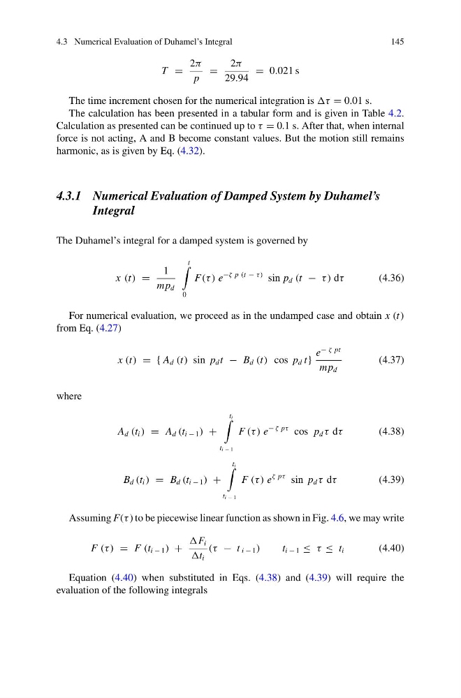
The Duhamel’s integral for a damped system is governed by
x (t) =
1
mp d
t
0
F(τ ) e
−ζ p (t − τ ) sin p d (t − τ ) dτ
(4.36)
For numerical evaluation, we proceed as in the undamped case and obtain x (t)
from Eq. (4.27)
x (t) = { A d (t) sin p d t − B d (t) cos p d t}
e
− ζ pt
mp d
(4.37)
where
A d (t i ) = A d (t i − 1 ) +
t i
t i − 1
F (τ ) e
− ζ pτ cos p d τ dτ
(4.38)
B d (t i ) = B d (t i − 1 ) +
t i
t i − 1
F (τ ) e
ζ pτ sin p d τ dτ
(4.39)
Assuming F(τ ) to be piecewise linear function as shown in Fig. 4.6, we may write
F (τ ) = F (t i − 1 ) +
F i
t i
(τ − t i − 1 )
t i − 1 ≤ τ ≤ t i
(4.40)
Equation (4.40) when substituted in Eqs. (4.38) and (4.39) will require the
evaluation of the following integrals
145
T =
2π
p
=
2π
29.94
= 0.021 s
The time increment chosen for the numerical integration is τ = 0.01 s.
The calculation has been presented in a tabular form and is given in Table 4.2.
Calculation as presented can be continued up to τ = 0.1 s. After that, when internal
force is not acting, A and B become constant values. But the motion still remains
harmonic, as is given by Eq. (4.32).
4.3.1 Numerical Evaluation of Damped System by Duhamel’s
Integral
The Duhamel’s integral for a damped system is governed by
x (t) =
1
mp d
t
0
F(τ ) e
−ζ p (t − τ ) sin p d (t − τ ) dτ
(4.36)
For numerical evaluation, we proceed as in the undamped case and obtain x (t)
from Eq. (4.27)
x (t) = { A d (t) sin p d t − B d (t) cos p d t}
e
− ζ pt
mp d
(4.37)
where
A d (t i ) = A d (t i − 1 ) +
t i
t i − 1
F (τ ) e
− ζ pτ cos p d τ dτ
(4.38)
B d (t i ) = B d (t i − 1 ) +
t i
t i − 1
F (τ ) e
ζ pτ sin p d τ dτ
(4.39)
Assuming F(τ ) to be piecewise linear function as shown in Fig. 4.6, we may write
F (τ ) = F (t i − 1 ) +
F i
t i
(τ − t i − 1 )
t i − 1 ≤ τ ≤ t i
(4.40)
Equation (4.40) when substituted in Eqs. (4.38) and (4.39) will require the
evaluation of the following integrals