

4.2 Direct Integration Techniques
139
˙
x = y
˙
y = f (x, y, t)
(4.20)
Assuming h = t, both x and y can be expressed in the terms of Taylor’s series
as
x = x i +
dx
dt
i
h +
d
2 x
dt 2
i
h
2
2
+ . . .
y = y i +
dy
dt
i
h +
d
2 y
dt 2
i
h
2
2
+ . . .
(4.21)
The expressions of Eq. (4.21) can be replaced in terms of the average slope by
neglecting higher-order derivatives
x = x i +
dx
dt
i av
h
y = y i +
dy
dt
i av
h
(4.22)
By using Simpson’s rule, the average slope in the interval h becomes,
dy
dt
i av
=
1
6
dy
dt
t i
+ 4
dy
dt
t i +
h
2
+
dy
dt
t i + h
(4.23)
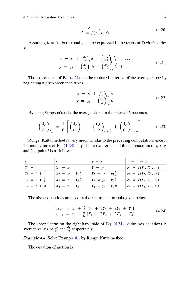
Runge–Kutta method is very much similar to the preceding computations except
the middle term of Eq. (4.23) is split into two terms and the computation of t, x, y,
and f at point i is as follows:
t
x
y = ˙
x
f = ˙
y = ¨
x
T 1 = t i
X 1 = x i
Y = y i
F 1 = f (T 1 , X 1 , Y 1 )
T 2 = t i +
h
2
X 2 = x i + Y 1
h
2
Y 2 = y i + F 1
h
2
F 2 = f (T 2 , X 2 , Y 2 )
T 3 = t i +
h
2
X 3 = x i + Y 2
h
2
Y 3 = y i + F 2
h
2
F 3 = f (T 3 , X 3 , Y 3 )
T 4 = t i + h
X 4 = x i + Y 3 h
Y 4 = y i + F 3 h
F 4 = f (T 4 , X 4 , Y 4 )
The above quantities are used in the recurrence formula given below:
x i + 1 = x i +
h
6
[Y 1 + 2Y 2 + 2Y 3 + Y 4 ]
y i + 1 = y i +
h
6
[F 1 + 2F 2 + 2F 3 + F 4 ]
(4.24)
The second term on the right-hand side of Eq. (4.24) of the two equations is
average values of
dx
dt
and
dy
dt
respectively.
Example 4.4 Solve Example 4.1 by Runge–Kutta method.
The equation of motion is
139
˙
x = y
˙
y = f (x, y, t)
(4.20)
Assuming h = t, both x and y can be expressed in the terms of Taylor’s series
as
x = x i +
dx
dt
i
h +
d
2 x
dt 2
i
h
2
2
+ . . .
y = y i +
dy
dt
i
h +
d
2 y
dt 2
i
h
2
2
+ . . .
(4.21)
The expressions of Eq. (4.21) can be replaced in terms of the average slope by
neglecting higher-order derivatives
x = x i +
dx
dt
i av
h
y = y i +
dy
dt
i av
h
(4.22)
By using Simpson’s rule, the average slope in the interval h becomes,
dy
dt
i av
=
1
6
dy
dt
t i
+ 4
dy
dt
t i +
h
2
+
dy
dt
t i + h
(4.23)
Runge–Kutta method is very much similar to the preceding computations except
the middle term of Eq. (4.23) is split into two terms and the computation of t, x, y,
and f at point i is as follows:
t
x
y = ˙
x
f = ˙
y = ¨
x
T 1 = t i
X 1 = x i
Y = y i
F 1 = f (T 1 , X 1 , Y 1 )
T 2 = t i +
h
2
X 2 = x i + Y 1
h
2
Y 2 = y i + F 1
h
2
F 2 = f (T 2 , X 2 , Y 2 )
T 3 = t i +
h
2
X 3 = x i + Y 2
h
2
Y 3 = y i + F 2
h
2
F 3 = f (T 3 , X 3 , Y 3 )
T 4 = t i + h
X 4 = x i + Y 3 h
Y 4 = y i + F 3 h
F 4 = f (T 4 , X 4 , Y 4 )
The above quantities are used in the recurrence formula given below:
x i + 1 = x i +
h
6
[Y 1 + 2Y 2 + 2Y 3 + Y 4 ]
y i + 1 = y i +
h
6
[F 1 + 2F 2 + 2F 3 + F 4 ]
(4.24)
The second term on the right-hand side of Eq. (4.24) of the two equations is
average values of
dx
dt
and
dy
dt
respectively.
Example 4.4 Solve Example 4.1 by Runge–Kutta method.
The equation of motion is