

138
4 Numerical Methods in Structural Dynamics …
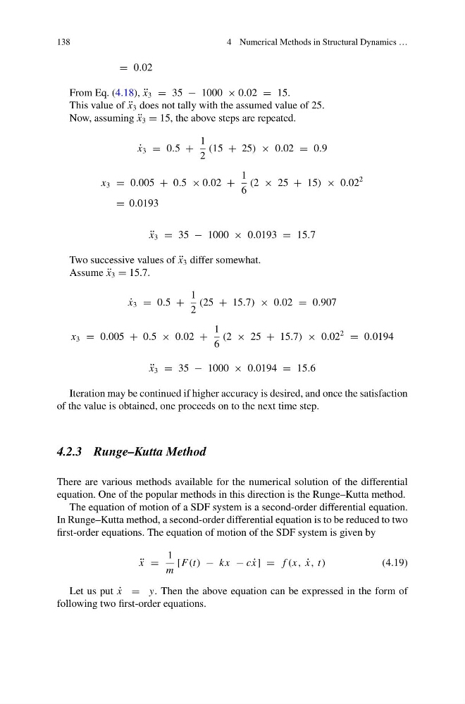
= 0.02
From Eq. (4.18), ¨
x 3 = 35 − 1000 × 0.02 = 15.
This value of ¨
x 3 does not tally with the assumed value of 25.
Now, assuming ¨
x 3 = 15, the above steps are repeated.
˙
x 3 = 0.5 +
1
2
(15 + 25) × 0.02 = 0.9
x 3 = 0.005 + 0.5 × 0.02 +
1
6
(2 × 25 + 15) × 0.02
2
= 0.0193
¨
x 3 = 35 − 1000 × 0.0193 = 15.7
Two successive values of ¨
x 3 differ somewhat.
Assume ¨
x 3 = 15.7.
˙
x 3 = 0.5 +
1
2
(25 + 15.7) × 0.02 = 0.907
x 3 = 0.005 + 0.5 × 0.02 +
1
6
(2 × 25 + 15.7) × 0.02
2
= 0.0194
¨
x 3 = 35 − 1000 × 0.0194 = 15.6
Iteration may be continued if higher accuracy is desired, and once the satisfaction
of the value is obtained, one proceeds on to the next time step.
4.2.3 Runge–Kutta Method
There are various methods available for the numerical solution of the differential
equation. One of the popular methods in this direction is the Runge–Kutta method.
The equation of motion of a SDF system is a second-order differential equation.
In Runge–Kutta method, a second-order differential equation is to be reduced to two
first-order equations. The equation of motion of the SDF system is given by
¨
x =
1
m
[F(t) − kx − c ˙
x] = f (x, ˙
x, t)
(4.19)
Let us put ˙
x = y. Then the above equation can be expressed in the form of
following two first-order equations.
4 Numerical Methods in Structural Dynamics …
= 0.02
From Eq. (4.18), ¨
x 3 = 35 − 1000 × 0.02 = 15.
This value of ¨
x 3 does not tally with the assumed value of 25.
Now, assuming ¨
x 3 = 15, the above steps are repeated.
˙
x 3 = 0.5 +
1
2
(15 + 25) × 0.02 = 0.9
x 3 = 0.005 + 0.5 × 0.02 +
1
6
(2 × 25 + 15) × 0.02
2
= 0.0193
¨
x 3 = 35 − 1000 × 0.0193 = 15.7
Two successive values of ¨
x 3 differ somewhat.
Assume ¨
x 3 = 15.7.
˙
x 3 = 0.5 +
1
2
(25 + 15.7) × 0.02 = 0.907
x 3 = 0.005 + 0.5 × 0.02 +
1
6
(2 × 25 + 15.7) × 0.02
2
= 0.0194
¨
x 3 = 35 − 1000 × 0.0194 = 15.6
Iteration may be continued if higher accuracy is desired, and once the satisfaction
of the value is obtained, one proceeds on to the next time step.
4.2.3 Runge–Kutta Method
There are various methods available for the numerical solution of the differential
equation. One of the popular methods in this direction is the Runge–Kutta method.
The equation of motion of a SDF system is a second-order differential equation.
In Runge–Kutta method, a second-order differential equation is to be reduced to two
first-order equations. The equation of motion of the SDF system is given by
¨
x =
1
m
[F(t) − kx − c ˙
x] = f (x, ˙
x, t)
(4.19)
Let us put ˙
x = y. Then the above equation can be expressed in the form of
following two first-order equations.