

140
4 Numerical Methods in Structural Dynamics …
¨
x =
1
2
F(t) − 1000x
Let y = ˙
x, then
˙
y = f (x, t) =
1
2
F(t) − 1000x
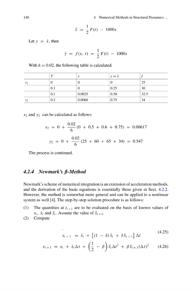
With h = 0.02, the following table is calculated.
T
x
y = ˙
x
f
t 1
0
0
0
25
0.1
0
0.25
30
0.1
0.0025
0.30
32.5
t 2
0.2
0.0060
0.75
34
x 2 and y 2 can be calculated as follows:
x 2 = 0 +
0.02
6
(0 + 0.5 + 0.6 + 0.75) = 0.00617
y 2 = 0 +
0.02
6
(25 + 60 + 65 + 34) = 0.547
The process is continued.
4.2.4 Newmark’s β-Method
Newmark’s scheme of numerical integration is an extension of acceleration methods,
and the derivation of the basic equations is essentially those given in Sect. 4.2.2.
However, the method is somewhat more general and can be applied to a nonlinear
system as well [4]. The step-by-step solution procedure is as follows:
(1) The quantities at t i + 1 are to be evaluated on the basis of known values of
x i , ˙
x i and ¨
x i . Assume the value of ¨
x i + 1 .
(2) Compute
.
x i + 1 = ˙
x i +
(1 − δ) ¨
x i + δ ¨
x i + 1
t
(4.25)
x i + 1 = x i + ˙
x i t +
1
2
− β
¨
x i t
2
+ β ¨
x i + 1 ( t)
2
(4.26)
4 Numerical Methods in Structural Dynamics …
¨
x =
1
2
F(t) − 1000x
Let y = ˙
x, then
˙
y = f (x, t) =
1
2
F(t) − 1000x
With h = 0.02, the following table is calculated.
T
x
y = ˙
x
f
t 1
0
0
0
25
0.1
0
0.25
30
0.1
0.0025
0.30
32.5
t 2
0.2
0.0060
0.75
34
x 2 and y 2 can be calculated as follows:
x 2 = 0 +
0.02
6
(0 + 0.5 + 0.6 + 0.75) = 0.00617
y 2 = 0 +
0.02
6
(25 + 60 + 65 + 34) = 0.547
The process is continued.
4.2.4 Newmark’s β-Method
Newmark’s scheme of numerical integration is an extension of acceleration methods,
and the derivation of the basic equations is essentially those given in Sect. 4.2.2.
However, the method is somewhat more general and can be applied to a nonlinear
system as well [4]. The step-by-step solution procedure is as follows:
(1) The quantities at t i + 1 are to be evaluated on the basis of known values of
x i , ˙
x i and ¨
x i . Assume the value of ¨
x i + 1 .
(2) Compute
.
x i + 1 = ˙
x i +
(1 − δ) ¨
x i + δ ¨
x i + 1
t
(4.25)
x i + 1 = x i + ˙
x i t +
1
2
− β
¨
x i t
2
+ β ¨
x i + 1 ( t)
2
(4.26)