

56
2 Experimental Methods for Determination of Nucleation Rates
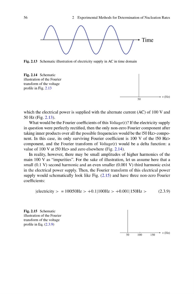
Fig. 2.13 Schematic illustration of electricity supply in AC in time domain
Fig. 2.14 Schematic
illustration of the Fourier
transform of the voltage
profile in Fig. 2.13
which the electrical power is supplied with the alternate current (AC) of 100 V and
50 Hz (Fig. 2.13).
What would be the Fourier coefficients of this Voltage(t)? If the electricity supply
in question were perfectly rectified, then the only non-zero Fourier component after
taking inner products over all the possible frequencies would be the |50 Hz> component. In this case, its only surviving Fourier coefficient is 100 V of the |50 Hz>
component, and the Fourier transform of Voltage(t) would be a delta function: a
value of 100 V at |50 Hz> and zero elsewhere (Fig. 2.14).
In reality, however, there may be small amplitudes of higher harmonics of the
main 100 V as “impurities”. For the sake of illustration, let us assume here that a
small (0.1 V) second harmonic and an even smaller (0.001 V) third harmonic exist
in the electrical power supply. Then, the Fourier transform of this electrical power
supply would schematically look like Fig. (2.15) and have three non-zero Fourier
coefficients:
|electricity > = 100|50Hz > +0.1|100Hz > +0.001|150Hz >
(2.3.9)
Fig. 2.15 Schematic
illustration of the Fourier
transform of the voltage
profile in Eq. (2.3.9)
2 Experimental Methods for Determination of Nucleation Rates
Fig. 2.13 Schematic illustration of electricity supply in AC in time domain
Fig. 2.14 Schematic
illustration of the Fourier
transform of the voltage
profile in Fig. 2.13
which the electrical power is supplied with the alternate current (AC) of 100 V and
50 Hz (Fig. 2.13).
What would be the Fourier coefficients of this Voltage(t)? If the electricity supply
in question were perfectly rectified, then the only non-zero Fourier component after
taking inner products over all the possible frequencies would be the |50 Hz> component. In this case, its only surviving Fourier coefficient is 100 V of the |50 Hz>
component, and the Fourier transform of Voltage(t) would be a delta function: a
value of 100 V at |50 Hz> and zero elsewhere (Fig. 2.14).
In reality, however, there may be small amplitudes of higher harmonics of the
main 100 V as “impurities”. For the sake of illustration, let us assume here that a
small (0.1 V) second harmonic and an even smaller (0.001 V) third harmonic exist
in the electrical power supply. Then, the Fourier transform of this electrical power
supply would schematically look like Fig. (2.15) and have three non-zero Fourier
coefficients:
|electricity > = 100|50Hz > +0.1|100Hz > +0.001|150Hz >
(2.3.9)
Fig. 2.15 Schematic
illustration of the Fourier
transform of the voltage
profile in Eq. (2.3.9)