2.3 Tea Time Break: The Fourier Transform and the Laplace Transform
57
2.3.3 The Laplace Transform
The trigonometric functions are not the only functions that form a Hilbert space of
infinite dimensions. As it turned out, exponential functions also form a Hilbert space
of infinite dimensions. That is, any one component, say exp(–x), cannot be expressed
in a linear combination of the other exponential functions such as exp(–2x). For
example,
| exp(−2x) > = α| exp(−3x) > +β| exp(−4x) >
(2.3.10)
Analogous to the Fourier transform in Eq. (2.3.8), the Laplace transform effectively “samples” an exponential component (decay constant) that is “parallel” to each
base:
F(s) ≡
∞
∫
0
f (t)e
−st dt
(2.3.11)
Here, F(s) is the Laplace transform and quantifies the “amplitude” or “amount”
that is “parallel” to each e
–st contained in f (t). The integrand in Eq. (2.3.11) is
effectively an inner product of f (t) with an exponential function e
–st , and such inner
product is integrated over every possible decay constant, s. In other words, Eq.
(2.3.11) effectively “samples” an exponential component that is “parallel” to each
base exponent and F(s) is the “amplitude” or “amount” of each such exponential
component (often referred to as Laplace s-domain).
Unlike the Fourier transform, though, the “infinite dimensions” of the Laplace
transform is limited to the half-space of negative exponent coefficients (the number
of the total dimensions is still infinite).
We may consider an example:
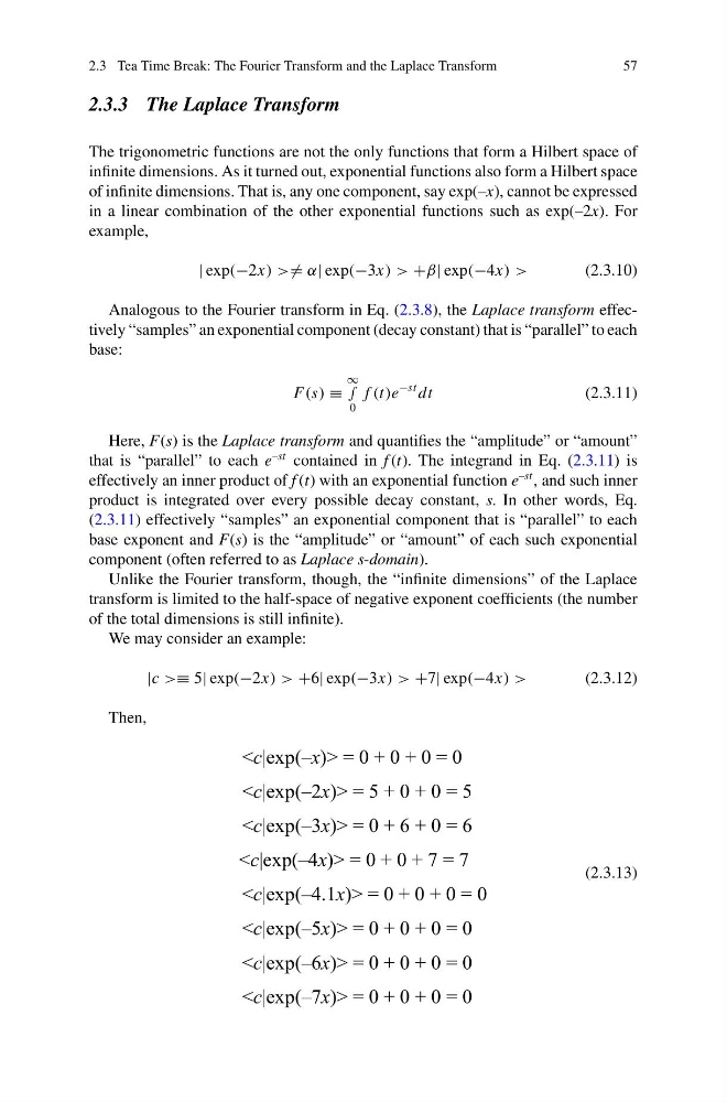
|c >≡ 5| exp(−2x) > +6| exp(−3x) > +7| exp(−4x) >
(2.3.12)
Then,
)> = 0 + 0 + 0 = 0
)> = 5 + 0 + 0 = 5
)> = 0 + 6 + 0 = 6
)> = 0 + 0 + 7 = 7
)> = 0 + 0 + 0 = 0
)> = 0 + 0 + 0 = 0
)> = 0 + 0 + 0 = 0
)> = 0 + 0 + 0 = 0
(2.3.13)