

48
2 Experimental Methods for Determination of Nucleation Rates
The nucleation probability density, p T (t), at each moment, t, is given by the
negative of the derivative of lnF T with respect to t, at that particular t and
the corresponding temperature (and subcooling), T. Then, just like we did in
Eq. (1.2.11),
k = p T (t)/ ln 2 ≈ p T (t)/0.7
(2.2.13)
We define the most probable lag time as the time at which the survival probability becomes 0.5 (i.e., when it is equally likely that a system has nucleated or not)
and define the nucleation rate as the inverse of the most probable lag time, k ≡ 1/
. To summarize, these analyses show that the nucleation probability density at a
given moment and subcooling during a linear cooling ramp only depends on the local
slope of the natural logarithm of the survival curve at that moment and subcooling.
2.2.4 Protocol of Converting an Experimentally Measured
Survival Curve to a Nucleation Curve
Now we are ready to put the above-described theoretical framework into practice.
One can construct a survival curve using an HP-ALTA or an HP-μDSC by assigning
measured fractions of samples or experimental runs that have nucleated at a given
temperature. A survival curve expresses the survival probability of the sample as a
function of the system subcooling, F = F(T ), which forms the starting point of
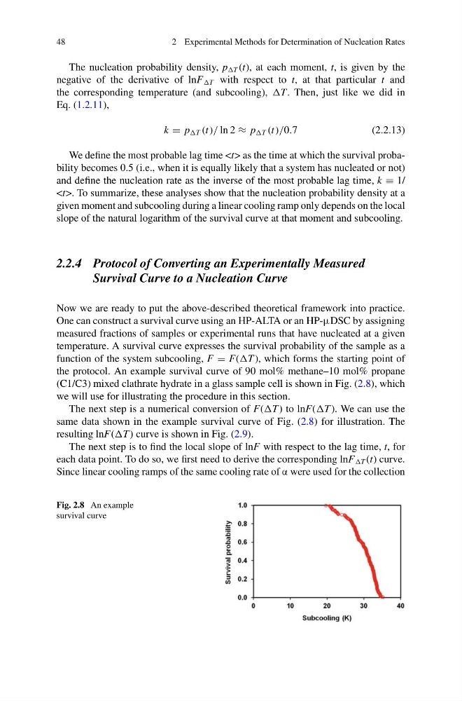
the protocol. An example survival curve of 90 mol% methane–10 mol% propane
(C1/C3) mixed clathrate hydrate in a glass sample cell is shown in Fig. (2.8), which
we will use for illustrating the procedure in this section.
The next step is a numerical conversion of F(T ) to lnF(T ). We can use the
same data shown in the example survival curve of Fig. (2.8) for illustration. The
resulting lnF(T ) curve is shown in Fig. (2.9).
The next step is to find the local slope of lnF with respect to the lag time, t, for
each data point. To do so, we first need to derive the corresponding lnF T (t) curve.
Since linear cooling ramps of the same cooling rate of α were used for the collection
Fig. 2.8 An example
survival curve
2 Experimental Methods for Determination of Nucleation Rates
The nucleation probability density, p T (t), at each moment, t, is given by the
negative of the derivative of lnF T with respect to t, at that particular t and
the corresponding temperature (and subcooling), T. Then, just like we did in
Eq. (1.2.11),
k = p T (t)/ ln 2 ≈ p T (t)/0.7
(2.2.13)
We define the most probable lag time
and define the nucleation rate as the inverse of the most probable lag time, k ≡ 1/
given moment and subcooling during a linear cooling ramp only depends on the local
slope of the natural logarithm of the survival curve at that moment and subcooling.
2.2.4 Protocol of Converting an Experimentally Measured
Survival Curve to a Nucleation Curve
Now we are ready to put the above-described theoretical framework into practice.
One can construct a survival curve using an HP-ALTA or an HP-μDSC by assigning
measured fractions of samples or experimental runs that have nucleated at a given
temperature. A survival curve expresses the survival probability of the sample as a
function of the system subcooling, F = F(T ), which forms the starting point of
the protocol. An example survival curve of 90 mol% methane–10 mol% propane
(C1/C3) mixed clathrate hydrate in a glass sample cell is shown in Fig. (2.8), which
we will use for illustrating the procedure in this section.
The next step is a numerical conversion of F(T ) to lnF(T ). We can use the
same data shown in the example survival curve of Fig. (2.8) for illustration. The
resulting lnF(T ) curve is shown in Fig. (2.9).
The next step is to find the local slope of lnF with respect to the lag time, t, for
each data point. To do so, we first need to derive the corresponding lnF T (t) curve.
Since linear cooling ramps of the same cooling rate of α were used for the collection
Fig. 2.8 An example
survival curve