

2.2 Linear Cooling Ramp Method
43
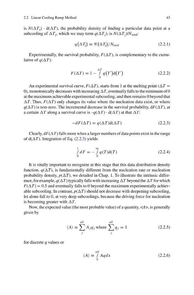
is N(T j ) · d(T ), the probability density of finding a particular data point at a
subcooling of T j , which we may term q(T j ), is N(T j )/N total :
q
T j
≡ N
T j
/N total
(2.2.1)
Experimentally, the survival probability, F(T ), is complementary to the cumulative of q(T ):
F((T ) = 1 −
T
∫
0
q
T
d
T
(2.2.2)
An experimental survival curve, F(T ), starts from 1 at the melting point (T =
0), monotonically decreases with increasing T, eventually falls to the minimum of 0
at the maximum achievable experimental subcooling, and then remains 0 beyond that
T. Thus, F(T ) only changes its value where the nucleation data exist, or where
q(T ) is non-zero. The incremental decrease in the survival probability, dF(T ), at
a certain T along a survival curve is –q(T ) · d(T ) at that T:
−dF((T ) = q((T )d((T )
(2.2.3)
Clearly, dF(T ) falls more when a larger numbers of data points exist in the range
of d(T ). Integration of Eq. (2.2.3) yields
1
∫
0
d F = −
∞
∫
0
q(T )d(T )
(2.2.4)
It is vitally important to recognize at this stage that this data distribution density
function, q(T ), is fundamentally different from the nucleation rate or nucleation
probability density, p(T ), we detailed in Chap. 1. To illustrate the intrinsic difference, for example, q(T ) typically falls with increasing T beyond the T for which
F(T ) = 0.5 and eventually falls to 0 beyond the maximum experimentally achievable subcooling. In contrast, p(T ) should not decrease with deepening subcooling,
let alone fall to 0, at very deep subcoolings, because the driving force for nucleation
is becoming greater with T.
Now, the expected value (the most probable value) of a quantity, , is generally
given by
A ≡
all
j
A j q j where
all
j
q j = 1
(2.2.5)
for discrete q values or
A ≡
all
∫
0
Aqd x
(2.2.6)
43
is N(T j ) · d(T ), the probability density of finding a particular data point at a
subcooling of T j , which we may term q(T j ), is N(T j )/N total :
q
T j
≡ N
T j
/N total
(2.2.1)
Experimentally, the survival probability, F(T ), is complementary to the cumulative of q(T ):
F((T ) = 1 −
T
∫
0
q
T
d
T
(2.2.2)
An experimental survival curve, F(T ), starts from 1 at the melting point (T =
0), monotonically decreases with increasing T, eventually falls to the minimum of 0
at the maximum achievable experimental subcooling, and then remains 0 beyond that
T. Thus, F(T ) only changes its value where the nucleation data exist, or where
q(T ) is non-zero. The incremental decrease in the survival probability, dF(T ), at
a certain T along a survival curve is –q(T ) · d(T ) at that T:
−dF((T ) = q((T )d((T )
(2.2.3)
Clearly, dF(T ) falls more when a larger numbers of data points exist in the range
of d(T ). Integration of Eq. (2.2.3) yields
1
∫
0
d F = −
∞
∫
0
q(T )d(T )
(2.2.4)
It is vitally important to recognize at this stage that this data distribution density
function, q(T ), is fundamentally different from the nucleation rate or nucleation
probability density, p(T ), we detailed in Chap. 1. To illustrate the intrinsic difference, for example, q(T ) typically falls with increasing T beyond the T for which
F(T ) = 0.5 and eventually falls to 0 beyond the maximum experimentally achievable subcooling. In contrast, p(T ) should not decrease with deepening subcooling,
let alone fall to 0, at very deep subcoolings, because the driving force for nucleation
is becoming greater with T.
Now, the expected value (the most probable value) of a quantity, , is generally
given by
A ≡
all
j
A j q j where
all
j
q j = 1
(2.2.5)
for discrete q values or
A ≡
all
∫
0
Aqd x
(2.2.6)