

44
2 Experimental Methods for Determination of Nucleation Rates
for continuous q values. By definition, q(T ) satisfies the condition of
all
j
q j = 1,
as per Eq. (2.2.1). Then, the most probable subcooling for which the distribution of
the data is given by q(T ) is
T =
∞
∫
0
T q(T )d(T )
(2.2.7)
Equation (2.2.7) can be simplified using Eq. (2.2.3):
T =
∞
∫
0
T q(T )d(T ) = −
∞
∫
0
T
d F
d(T )
d(T ) =
1
∫
0
T d F
(2.2.8)
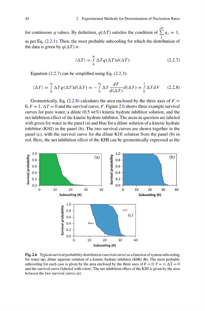
Geometrically, Eq. (2.2.8) calculates the area enclosed by the three axes of F =
0, F = 1, T = 0 and the survival curve, F. Figure 2.6 shows three example survival
curves for pure water, a dilute (0.5 wt%) kinetic hydrate inhibitor solution, and the
net inhibition effect of the kinetic hydrate inhibitor. The areas in question are labeled
with green for water in the panel (a) and blue for a dilute solution of a kinetic hydrate
inhibitor (KHI) in the panel (b). The two survival curves are shown together in the
panel (c), with the survival curve for the dilute KHI solution from the panel (b) in
red. Here, the net inhibition effect of the KHI can be geometrically expressed as the
Fig. 2.6 Typical survival probability distribution (survival curve) as a function of system subcooling
for water (a), dilute aqueous solution of a kinetic hydrate inhibitor (KHI) (b). The most probable
subcooling for each case is given by the area enclosed by the three axes of F = 0, F = 1, T = 0
and the survival curve (labeled with color). The net inhibition effect of the KHI is given by the area
between the two survival curves (c)
2 Experimental Methods for Determination of Nucleation Rates
for continuous q values. By definition, q(T ) satisfies the condition of
all
j
q j = 1,
as per Eq. (2.2.1). Then, the most probable subcooling for which the distribution of
the data is given by q(T ) is
T =
∞
∫
0
T q(T )d(T )
(2.2.7)
Equation (2.2.7) can be simplified using Eq. (2.2.3):
T =
∞
∫
0
T q(T )d(T ) = −
∞
∫
0
T
d F
d(T )
d(T ) =
1
∫
0
T d F
(2.2.8)
Geometrically, Eq. (2.2.8) calculates the area enclosed by the three axes of F =
0, F = 1, T = 0 and the survival curve, F. Figure 2.6 shows three example survival
curves for pure water, a dilute (0.5 wt%) kinetic hydrate inhibitor solution, and the
net inhibition effect of the kinetic hydrate inhibitor. The areas in question are labeled
with green for water in the panel (a) and blue for a dilute solution of a kinetic hydrate
inhibitor (KHI) in the panel (b). The two survival curves are shown together in the
panel (c), with the survival curve for the dilute KHI solution from the panel (b) in
red. Here, the net inhibition effect of the KHI can be geometrically expressed as the
Fig. 2.6 Typical survival probability distribution (survival curve) as a function of system subcooling
for water (a), dilute aqueous solution of a kinetic hydrate inhibitor (KHI) (b). The most probable
subcooling for each case is given by the area enclosed by the three axes of F = 0, F = 1, T = 0
and the survival curve (labeled with color). The net inhibition effect of the KHI is given by the area
between the two survival curves (c)