

7.3.3 3D Edge Plasma Turbulence Modeling
Today, quite a few codes of different sophistication are available for edge plasma
turbulence simulation: BOUT++ [147], XGC1 [106], TOKAM3X [141], GBS
[142], GDB [31], GRILLIX [143], Gkeyll [108], and some others.
These codes are used for both modeling some particular experiments and for
studying the general characteristics and dependences of edge plasma turbulence. For
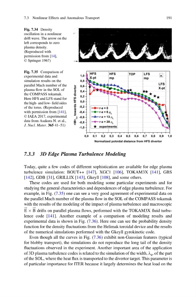
example, in Fig. (7.35) one can see a very good agreement of experimental data on
the parallel Mach number of the plasma flow in the SOL of the COMPASS tokamak
with the results of the modeling of the impact of plasma turbulence and macroscopic
E
! Â B
!
drifts on parallel plasma flows, performed with the TOKAM3X fluid turbulence code [141]. Another example of a comparison of modeling results and
experimental data is shown in Fig. (7.36). Here one can see the probability density
function for the density fluctuations from the Helimak toroidal device and the results
of the numerical simulations performed with the Gkeyll gyrokinetic code.
Even though all the curves in Fig. (7.36) exhibit non-Gaussian features (typical
for blobby transport), the simulations do not reproduce the long tail of the density
fluctuations observed in the experiment. Another important area of the application
of 3D plasma turbulence codes is related to the simulation of the width, λ q , of the part
of the SOL, where the heat flux is transported to the divertor target. This parameter is
of particular importance for ITER because it largely determines the heat load on the
Fig. 7.34 Density
oscillation in a nonlinear
drift wave. The arrow on the
left corresponds to zero
plasma density.
(Reproduced with
permission from [14],
© Springer 1967)
Fig. 7.35 Comparison of
experimental data and
simulation results on the
parallel Mach number of the
plasma flow in the SOL of
the COMPASS tokamak.
Here HFS and LFS stand for
the high- and low- field sides
of the torus. (Reproduced
with permission from [141],
© IAEA 2017, experimental
data from Asakura N. et al.,
J. Nucl. Mater. 365 41–51)
7.3 Nonlinear Effects and Anomalous Transport
191
Today, quite a few codes of different sophistication are available for edge plasma
turbulence simulation: BOUT++ [147], XGC1 [106], TOKAM3X [141], GBS
[142], GDB [31], GRILLIX [143], Gkeyll [108], and some others.
These codes are used for both modeling some particular experiments and for
studying the general characteristics and dependences of edge plasma turbulence. For
example, in Fig. (7.35) one can see a very good agreement of experimental data on
the parallel Mach number of the plasma flow in the SOL of the COMPASS tokamak
with the results of the modeling of the impact of plasma turbulence and macroscopic
E
! Â B
!
drifts on parallel plasma flows, performed with the TOKAM3X fluid turbulence code [141]. Another example of a comparison of modeling results and
experimental data is shown in Fig. (7.36). Here one can see the probability density
function for the density fluctuations from the Helimak toroidal device and the results
of the numerical simulations performed with the Gkeyll gyrokinetic code.
Even though all the curves in Fig. (7.36) exhibit non-Gaussian features (typical
for blobby transport), the simulations do not reproduce the long tail of the density
fluctuations observed in the experiment. Another important area of the application
of 3D plasma turbulence codes is related to the simulation of the width, λ q , of the part
of the SOL, where the heat flux is transported to the divertor target. This parameter is
of particular importance for ITER because it largely determines the heat load on the
Fig. 7.34 Density
oscillation in a nonlinear
drift wave. The arrow on the
left corresponds to zero
plasma density.
(Reproduced with
permission from [14],
© Springer 1967)
Fig. 7.35 Comparison of
experimental data and
simulation results on the
parallel Mach number of the
plasma flow in the SOL of
the COMPASS tokamak.
Here HFS and LFS stand for
the high- and low- field sides
of the torus. (Reproduced
with permission from [141],
© IAEA 2017, experimental
data from Asakura N. et al.,
J. Nucl. Mater. 365 41–51)
7.3 Nonlinear Effects and Anomalous Transport
191