

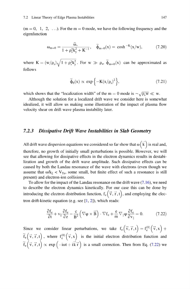
(m ¼ 0, 1, 2, . . .). For the m ¼ 0 mode, we have the following frequency and the
eigenfunction
ω m¼0 ¼
b
ω Ã
1 þ ρ 2
s k
2
y þ K
À1
, e
ϕ m¼0 x
ð Þ ¼ cosh
ÀK x=w
ð
Þ,
ð7:20Þ
where K ¼ w=ρ s
ð
Þ
ffiffiffiffiffiffiffiffiffiffiffiffiffiffiffiffiffi
1 þ ρ 2
s k
2
y
q
. For w ) ρ s , e
ϕ m¼0 x
ð Þ can be approximated as
follows
e
ϕ 0 x
ð Þ / exp ÀK x=ρ s
ð
Þ
2
n
o
,
ð7:21Þ
which shows that the “localization width” of the m ¼ 0 mode is ∼
ffiffiffiffiffiffiffi ffi
ρ s w
p
( w.
Although the solution for a localized drift wave we consider here is somewhat
idealized, it will allow us making some illustration of the impact of plasma flow
velocity shear on drift wave plasma instability later.
7.2.3 Dissipative Drift Wave Instabilities in Slab Geometry
All drift wave dispersion equations we considered so far show that ω k
!
is real and,
therefore, no growth of initially small perturbations is possible. However, we will
see that allowing for dissipative effects in the electron dynamics results in destabilization and growth of the drift wave amplitude. Such dissipative effects can be
caused by both the Landau resonance of the wave with electrons (even though we
assume that ω/k k < V Te , some small, but finite effect of such a resonance is still
present) and electron-ion collisions.
To allow for the impact of the Landau resonance on the drift wave (7.16), we need
to describe the electron dynamics kinetically. For our case this can be done by
introducing the electron distribution function, f e v
!
, r
!
, t
, and employing the electron drift-kinetic equation (e.g. see [1, 2]), which reads:
∂f e
∂t
þ v k
∂f e
∂z
À
c
B
2
∇φ Â B
!
Á ∇f e þ
e
m
∇ k φ
∂f e
∂v k
¼ 0:
ð7:22Þ
Since we consider linear perturbations, we take f e v
!
, r
!
, t
¼ f
0
ð Þ
e
v
!
, x
þ
e f e v
!
, r
!
, t
, where f
0
ð Þ
e
v
!
, x
is the initial electron distribution function and
e f e v
!
, r
!
, t
/ exp Àiωt þ ik
!
r
!
is a small correction. Then from Eq. (7.22) we
7.2 Linear Theory of Edge Plasma Instabilities
147
eigenfunction
ω m¼0 ¼
b
ω Ã
1 þ ρ 2
s k
2
y þ K
À1
, e
ϕ m¼0 x
ð Þ ¼ cosh
ÀK x=w
ð
Þ,
ð7:20Þ
where K ¼ w=ρ s
ð
Þ
ffiffiffiffiffiffiffiffiffiffiffiffiffiffiffiffiffi
1 þ ρ 2
s k
2
y
q
. For w ) ρ s , e
ϕ m¼0 x
ð Þ can be approximated as
follows
e
ϕ 0 x
ð Þ / exp ÀK x=ρ s
ð
Þ
2
n
o
,
ð7:21Þ
which shows that the “localization width” of the m ¼ 0 mode is ∼
ffiffiffiffiffiffiffi ffi
ρ s w
p
( w.
Although the solution for a localized drift wave we consider here is somewhat
idealized, it will allow us making some illustration of the impact of plasma flow
velocity shear on drift wave plasma instability later.
7.2.3 Dissipative Drift Wave Instabilities in Slab Geometry
All drift wave dispersion equations we considered so far show that ω k
!
is real and,
therefore, no growth of initially small perturbations is possible. However, we will
see that allowing for dissipative effects in the electron dynamics results in destabilization and growth of the drift wave amplitude. Such dissipative effects can be
caused by both the Landau resonance of the wave with electrons (even though we
assume that ω/k k < V Te , some small, but finite effect of such a resonance is still
present) and electron-ion collisions.
To allow for the impact of the Landau resonance on the drift wave (7.16), we need
to describe the electron dynamics kinetically. For our case this can be done by
introducing the electron distribution function, f e v
!
, r
!
, t
, and employing the electron drift-kinetic equation (e.g. see [1, 2]), which reads:
∂f e
∂t
þ v k
∂f e
∂z
À
c
B
2
∇φ Â B
!
Á ∇f e þ
e
m
∇ k φ
∂f e
∂v k
¼ 0:
ð7:22Þ
Since we consider linear perturbations, we take f e v
!
, r
!
, t
¼ f
0
ð Þ
e
v
!
, x
þ
e f e v
!
, r
!
, t
, where f
0
ð Þ
e
v
!
, x
is the initial electron distribution function and
e f e v
!
, r
!
, t
/ exp Àiωt þ ik
!
r
!
is a small correction. Then from Eq. (7.22) we
7.2 Linear Theory of Edge Plasma Instabilities
147