

various atomic processes such as ionization, charge-exchange, and others. The
electric, E
!
, and magnetic, B
!
, fields in Eq. (6.1) need to be determined selfconsistently from the Maxwell equations with the electric charges and current
sources found from the solution of the kinetic equations (6.1). Solving all these
equations can only be possible numerically. However, in the near future, this is not
feasible without a significant reduction of these equations. In general, the fluid
equations themselves are the examples of such a reduction when the time evolution
of the six-dimensional distribution function is replaced by a truncated set of
nonlinear equations for space and time evolution of the moments, b
M r
!
, t
, of the
distribution function f α
v
!
, r
!
, t
, defined as the integrals b
M
r
!
, t
¼
R b b
M
v
!
f α
v
! , r
!
, t
dv
! . We notice that in general case, both
b b
M v
!
and b
M r
! , t
can be tensors. The first moments of a distribution function F
v
!
, r
!
, t
are the basic
fluid variables such as the particle density, n r
!
, t
, the average (fluid) velocity,
V
!
r
!
, t
, and the pressure, p r
!
, t
, that have simple macroscopic meaning:
n
r
!
, t
¼
Z
F
v
! , r
!
, t
dv
!
,
ð6:2Þ
n
r
!
, t
V
!
r
! , t
¼
Z
v
!
F
v
!
, r
!
, t
dv
! ,
ð6:3Þ
p r
!
, t
¼
m
3
Z
v
0 2 F v
0
!
, r
!
, t
dv
!
,
ð6:4Þ
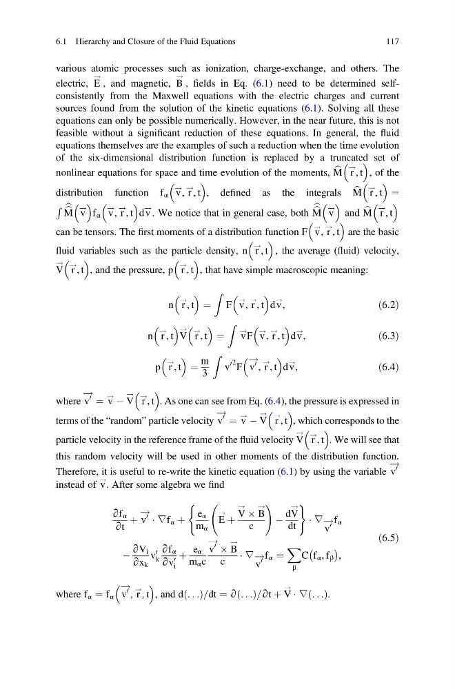
where v
0
! ¼ v
! À V
!
r
! , t
. As one can see from Eq. (6.4), the pressure is expressed in
terms of the “random” particle velocity v
0
! ¼ v
! À V
!
r
! , t
, which corresponds to the
particle velocity in the reference frame of the fluid velocity V
!
r
!
, t
. We will see that
this random velocity will be used in other moments of the distribution function.
Therefore, it is useful to re-write the kinetic equation (6.1) by using the variable v
0
!
instead of v
!
. After some algebra we find
∂f α
∂t
þ v
0
! Á ∇f α þ
e α
m α
E
! þ
V
! Â B
!
c
!
À
dV
!
dt
(
)
Á ∇
v
0
!fα
À
∂V i
∂x k
v
0
k
∂f α
∂v 0
i
þ
e α
m α c
v
0
! Â B
!
c
Á ∇
v
0
!fα ¼
X
β
C f α , f β
À
Á
,
ð6:5Þ
where f α ¼ f α v
0
!
, r
!
, t
, and d . . .
ð Þ=dt ¼ ∂ . . .
ð Þ=∂t þ V
! Á ∇ . . .
ð Þ.
6.1 Hierarchy and Closure of the Fluid Equations
117
electric, E
!
, and magnetic, B
!
, fields in Eq. (6.1) need to be determined selfconsistently from the Maxwell equations with the electric charges and current
sources found from the solution of the kinetic equations (6.1). Solving all these
equations can only be possible numerically. However, in the near future, this is not
feasible without a significant reduction of these equations. In general, the fluid
equations themselves are the examples of such a reduction when the time evolution
of the six-dimensional distribution function is replaced by a truncated set of
nonlinear equations for space and time evolution of the moments, b
M r
!
, t
, of the
distribution function f α
v
!
, r
!
, t
, defined as the integrals b
M
r
!
, t
¼
R b b
M
v
!
f α
v
! , r
!
, t
dv
! . We notice that in general case, both
b b
M v
!
and b
M r
! , t
can be tensors. The first moments of a distribution function F
v
!
, r
!
, t
are the basic
fluid variables such as the particle density, n r
!
, t
, the average (fluid) velocity,
V
!
r
!
, t
, and the pressure, p r
!
, t
, that have simple macroscopic meaning:
n
r
!
, t
¼
Z
F
v
! , r
!
, t
dv
!
,
ð6:2Þ
n
r
!
, t
V
!
r
! , t
¼
Z
v
!
F
v
!
, r
!
, t
dv
! ,
ð6:3Þ
p r
!
, t
¼
m
3
Z
v
0 2 F v
0
!
, r
!
, t
dv
!
,
ð6:4Þ
where v
0
! ¼ v
! À V
!
r
! , t
. As one can see from Eq. (6.4), the pressure is expressed in
terms of the “random” particle velocity v
0
! ¼ v
! À V
!
r
! , t
, which corresponds to the
particle velocity in the reference frame of the fluid velocity V
!
r
!
, t
. We will see that
this random velocity will be used in other moments of the distribution function.
Therefore, it is useful to re-write the kinetic equation (6.1) by using the variable v
0
!
instead of v
!
. After some algebra we find
∂f α
∂t
þ v
0
! Á ∇f α þ
e α
m α
E
! þ
V
! Â B
!
c
!
À
dV
!
dt
(
)
Á ∇
v
0
!fα
À
∂V i
∂x k
v
0
k
∂f α
∂v 0
i
þ
e α
m α c
v
0
! Â B
!
c
Á ∇
v
0
!fα ¼
X
β
C f α , f β
À
Á
,
ð6:5Þ
where f α ¼ f α v
0
!
, r
!
, t
, and d . . .
ð Þ=dt ¼ ∂ . . .
ð Þ=∂t þ V
! Á ∇ . . .
ð Þ.
6.1 Hierarchy and Closure of the Fluid Equations
117