

152
5 Two-Dimensional Problems in Cartesian Co-ordinate System
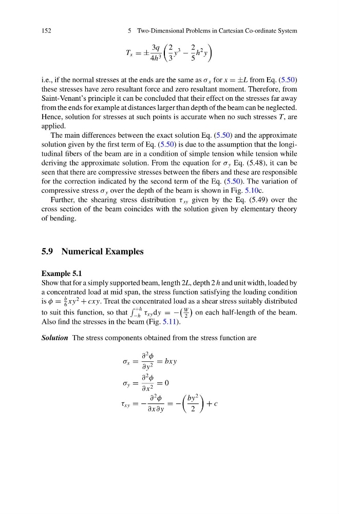
T x = ±
3q
4h 3
2
3
y
3
−
2
5
h
2 y
i.e., if the normal stresses at the ends are the same as σ x for x = ±L from Eq. (5.50)
these stresses have zero resultant force and zero resultant moment. Therefore, from
Saint-Venant’s principle it can be concluded that their effect on the stresses far away
from the ends for example at distances larger than depth of the beam can be neglected.
Hence, solution for stresses at such points is accurate when no such stresses T, are
applied.
The main differences between the exact solution Eq. (5.50) and the approximate
solution given by the first term of Eq. (5.50) is due to the assumption that the longitudinal fibers of the beam are in a condition of simple tension while tension while
deriving the approximate solution. From the equation for σ y Eq. (5.48), it can be
seen that there are compressive stresses between the fibers and these are responsible
for the correction indicated by the second term of the Eq. (5.50). The variation of
compressive stress σ y over the depth of the beam is shown in Fig. 5.10c.
Further, the shearing stress distribution τ xy given by the Eq. (5.49) over the
cross section of the beam coincides with the solution given by elementary theory
of bending.
5.9 Numerical Examples
Example 5.1
Show that for a simply supported beam, length 2L, depth 2 h and unit width, loaded by
a concentrated load at mid span, the stress function satisfying the loading condition
is φ =
b
6
x y
2
+ cx y. Treat the concentrated load as a shear stress suitably distributed
to suit this function, so that
+h
−h τ xy dy = −
W
2
on each half-length of the beam.
Also find the stresses in the beam (Fig. 5.11).
Solution The stress components obtained from the stress function are
σ x =
∂
2
φ
∂ y 2 = bx y
σ y =
∂
2
φ
∂ x 2 = 0
τ xy = −
∂
2
φ
∂ x∂ y
= −
by
2
2
+ c
5 Two-Dimensional Problems in Cartesian Co-ordinate System
T x = ±
3q
4h 3
2
3
y
3
−
2
5
h
2 y
i.e., if the normal stresses at the ends are the same as σ x for x = ±L from Eq. (5.50)
these stresses have zero resultant force and zero resultant moment. Therefore, from
Saint-Venant’s principle it can be concluded that their effect on the stresses far away
from the ends for example at distances larger than depth of the beam can be neglected.
Hence, solution for stresses at such points is accurate when no such stresses T, are
applied.
The main differences between the exact solution Eq. (5.50) and the approximate
solution given by the first term of Eq. (5.50) is due to the assumption that the longitudinal fibers of the beam are in a condition of simple tension while tension while
deriving the approximate solution. From the equation for σ y Eq. (5.48), it can be
seen that there are compressive stresses between the fibers and these are responsible
for the correction indicated by the second term of the Eq. (5.50). The variation of
compressive stress σ y over the depth of the beam is shown in Fig. 5.10c.
Further, the shearing stress distribution τ xy given by the Eq. (5.49) over the
cross section of the beam coincides with the solution given by elementary theory
of bending.
5.9 Numerical Examples
Example 5.1
Show that for a simply supported beam, length 2L, depth 2 h and unit width, loaded by
a concentrated load at mid span, the stress function satisfying the loading condition
is φ =
b
6
x y
2
+ cx y. Treat the concentrated load as a shear stress suitably distributed
to suit this function, so that
+h
−h τ xy dy = −
W
2
on each half-length of the beam.
Also find the stresses in the beam (Fig. 5.11).
Solution The stress components obtained from the stress function are
σ x =
∂
2
φ
∂ y 2 = bx y
σ y =
∂
2
φ
∂ x 2 = 0
τ xy = −
∂
2
φ
∂ x∂ y
= −
by
2
2
+ c