

120
5 General-Relativistic Matrix Kinetic Theory
∼
a
r1
b
r
1
f s2s
2
f r2r
2
f
◦
s
1 s1 f
◦
r
1 r
1
A(γ r2 , e s2 → γ r1 , e s1 ) A
∗ (γ r
2
, e s
2
→ γ r
1
, e s
1
)
=
a
r1
b
r
1
f s2s
2
f r2r
2
f
◦
s
1 s1 f
◦
r
1 r
1
c
r1
d
r2 ¯
u s1 A cd (k 1 , k 2 , p 1 , p 2 ) u s2
e
r
1
f
r
2
¯
u s
2
¯
A ef (k 1 , k 2 , p 1 , p 2 ) u s
1
≡ (
a
r1
c
r1 ) ( f r2r
2
d
r2
f
r
2
) ( f
◦
r
1 r
1
e
r
1
b
r
1
)
× Tr
A cd (k 1 , k 2 , p 1 , p 2 ) (u s2 f s2s
2
¯
u s
2
) ¯
A ef (k 1 , k 2 , p 1 , p 2 ) (u s
1
f
◦
s
1 s1 ¯
u s1 )
≡ 4m
2
e
a f
1 f
cd
2 f
◦,eb
1
Tr
A f c (k 1 , k 2 , p 1 , p 2 ) f e,2 ¯
A ed (k 1 , k 2 , p 1 , p 2 ) f
◦
e,1
.
(5.10.19)
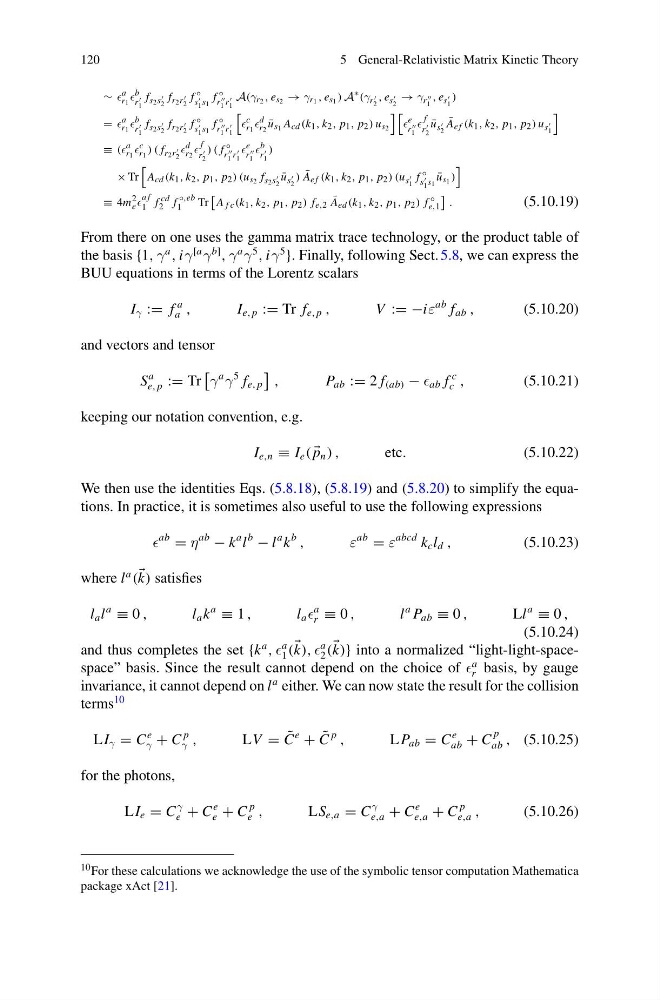
From there on one uses the gamma matrix trace technology, or the product table of
the basis {1, γ
a
, iγ
[a
γ
b]
, γ
a
γ
5
, iγ
5
}. Finally, following Sect. 5.8, we can express the
BUU equations in terms of the Lorentz scalars
I γ := f
a
a ,
I e, p := Tr f e, p ,
V := −iε
ab f ab ,
(5.10.20)
and vectors and tensor
S
a
e, p := Tr
γ
a
γ
5 f e, p
,
P ab := 2 f (ab) − ab f
c
c ,
(5.10.21)
keeping our notation convention, e.g.
I e,n ≡ I e (
p n ) ,
etc.
(5.10.22)
We then use the identities Eqs. (5.8.18), (5.8.19) and (5.8.20) to simplify the equations. In practice, it is sometimes also useful to use the following expressions
ab
= η
ab
− k
a l
b
− l
a k
b
,
ε
ab
= ε
abcd k c l d ,
(5.10.23)
where l
a
(
k) satisfies
l a l
a
≡ 0 ,
l a k
a
≡ 1 ,
l a
a
r ≡ 0 ,
l
a P ab ≡ 0 ,
Ll
a
≡ 0 ,
(5.10.24)
and thus completes the set {k
a
,
a
1 (
k),
a
2 (
k)} into a normalized “light-light-spacespace” basis. Since the result cannot depend on the choice of
a
r basis, by gauge
invariance, it cannot depend on l
a either. We can now state the result for the collision
terms
10
LI γ = C
e
γ + C
p
γ ,
LV = ˜
C
e
+ ˜
C
p
,
L P ab = C
e
ab + C
p
ab , (5.10.25)
for the photons,
LI e = C
γ
e + C
e
e + C
p
e ,
LS e,a = C
γ
e,a + C
e
e,a + C
p
e,a ,
(5.10.26)
10 For these calculations we acknowledge the use of the symbolic tensor computation Mathematica
package xAct [21].
5 General-Relativistic Matrix Kinetic Theory
∼
a
r1
b
r
1
f s2s
2
f r2r
2
f
◦
s
1 s1 f
◦
r
1 r
1
A(γ r2 , e s2 → γ r1 , e s1 ) A
∗ (γ r
2
, e s
2
→ γ r
1
, e s
1
)
=
a
r1
b
r
1
f s2s
2
f r2r
2
f
◦
s
1 s1 f
◦
r
1 r
1
c
r1
d
r2 ¯
u s1 A cd (k 1 , k 2 , p 1 , p 2 ) u s2
e
r
1
f
r
2
¯
u s
2
¯
A ef (k 1 , k 2 , p 1 , p 2 ) u s
1
≡ (
a
r1
c
r1 ) ( f r2r
2
d
r2
f
r
2
) ( f
◦
r
1 r
1
e
r
1
b
r
1
)
× Tr
A cd (k 1 , k 2 , p 1 , p 2 ) (u s2 f s2s
2
¯
u s
2
) ¯
A ef (k 1 , k 2 , p 1 , p 2 ) (u s
1
f
◦
s
1 s1 ¯
u s1 )
≡ 4m
2
e
a f
1 f
cd
2 f
◦,eb
1
Tr
A f c (k 1 , k 2 , p 1 , p 2 ) f e,2 ¯
A ed (k 1 , k 2 , p 1 , p 2 ) f
◦
e,1
.
(5.10.19)
From there on one uses the gamma matrix trace technology, or the product table of
the basis {1, γ
a
, iγ
[a
γ
b]
, γ
a
γ
5
, iγ
5
}. Finally, following Sect. 5.8, we can express the
BUU equations in terms of the Lorentz scalars
I γ := f
a
a ,
I e, p := Tr f e, p ,
V := −iε
ab f ab ,
(5.10.20)
and vectors and tensor
S
a
e, p := Tr
γ
a
γ
5 f e, p
,
P ab := 2 f (ab) − ab f
c
c ,
(5.10.21)
keeping our notation convention, e.g.
I e,n ≡ I e (
p n ) ,
etc.
(5.10.22)
We then use the identities Eqs. (5.8.18), (5.8.19) and (5.8.20) to simplify the equations. In practice, it is sometimes also useful to use the following expressions
ab
= η
ab
− k
a l
b
− l
a k
b
,
ε
ab
= ε
abcd k c l d ,
(5.10.23)
where l
a
(
k) satisfies
l a l
a
≡ 0 ,
l a k
a
≡ 1 ,
l a
a
r ≡ 0 ,
l
a P ab ≡ 0 ,
Ll
a
≡ 0 ,
(5.10.24)
and thus completes the set {k
a
,
a
1 (
k),
a
2 (
k)} into a normalized “light-light-spacespace” basis. Since the result cannot depend on the choice of
a
r basis, by gauge
invariance, it cannot depend on l
a either. We can now state the result for the collision
terms
10
LI γ = C
e
γ + C
p
γ ,
LV = ˜
C
e
+ ˜
C
p
,
L P ab = C
e
ab + C
p
ab , (5.10.25)
for the photons,
LI e = C
γ
e + C
e
e + C
p
e ,
LS e,a = C
γ
e,a + C
e
e,a + C
p
e,a ,
(5.10.26)
10 For these calculations we acknowledge the use of the symbolic tensor computation Mathematica
package xAct [21].