

5.10 Example: The Photon-Electron-Proton Fluid
119
iA(e s3 , e s4 → e s1 , e s2 ) :=
+
= −
i
2
e
2
¯
u s 1 γ a u s 3 ¯
u s 2 γ
a u s 4
m 2
e + p 1 · p 3
−
¯
u s 1 γ a u s 4 ¯
u s 2 γ
a u s 3
m 2
e + p 1 · p 4
,
(5.10.16)
iA(e s2 , p t2 → e s1 , p t1 ) :=
=
i
2
e
2 ¯
u s 1 γ a u s 2 ¯
u t 1 γ
a u t 2
m 2
e + p 1 · p 2
,
(5.10.17)
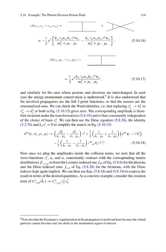
and similarly for the ones where protons and electrons are interchanged. In each
case the energy-momentum conservation is understood.
9 It is also understood that
the involved propagators are the full 2-point functions, so that the masses are the
renormalized ones. We can check the Ward identities, i.e. that replacing
a
r 1
→ k
a
1 or
b
r 2
→ k
b
2 or both in Eq. (5.10.15) gives zero. The corresponding amplitude is therefore invariant under the transformations (5.8.10) and is thus consistently independent
of the choice of basis
a
r . We can then use the Dirac equation (5.8.26), the identity
(3.2.76) and k a
a
r ≡ 0 to simplify the matrix in Eq. (5.10.15)
A
ab (k 1 , k 2 , p 1 , p 2 ) →
p a
2
k 1 · p 2
−
p a
1
k 1 · p 1
γ
b +
1
2
1
k 1 · p 1
+
1
k 1 · p 2
η
ab
k 1 − γ
a k
b
1
−
i
2
1
k 1 · p 1
−
1
k 1 · p 2
ε
ab
cd k
c
1 γ
d γ
5 .
(5.10.18)
Now once we plug the amplitudes inside the collision terms, we note that all the
wave-functions
a
r , u s and u t consistently contract with the corresponding matrix
distributions f γ,e, p to form the Lorentz-indexed one f ab of Eq. (5.8.6) for the photons
and the Dirac-indexed ones f e, p of Eq. (5.8.28) for the fermions, with the Dirac
indexes kept again implicit. We can then use Eqs. (5.8.16) and (5.8.34) to express the
result in terms of the desired quantities. As a concrete example, consider the creation
term of C
e
γ,ab (
k 1 ) := C
e
γ,r 1 r
1
r 1
a
r
1
b
9 Note also that the Feynman i regularization in the propagators is irrelevant here because the virtual
particles cannot become real (on-shell) in the momentum region of interest.
119
iA(e s3 , e s4 → e s1 , e s2 ) :=
+
= −
i
2
e
2
¯
u s 1 γ a u s 3 ¯
u s 2 γ
a u s 4
m 2
e + p 1 · p 3
−
¯
u s 1 γ a u s 4 ¯
u s 2 γ
a u s 3
m 2
e + p 1 · p 4
,
(5.10.16)
iA(e s2 , p t2 → e s1 , p t1 ) :=
=
i
2
e
2 ¯
u s 1 γ a u s 2 ¯
u t 1 γ
a u t 2
m 2
e + p 1 · p 2
,
(5.10.17)
and similarly for the ones where protons and electrons are interchanged. In each
case the energy-momentum conservation is understood.
9 It is also understood that
the involved propagators are the full 2-point functions, so that the masses are the
renormalized ones. We can check the Ward identities, i.e. that replacing
a
r 1
→ k
a
1 or
b
r 2
→ k
b
2 or both in Eq. (5.10.15) gives zero. The corresponding amplitude is therefore invariant under the transformations (5.8.10) and is thus consistently independent
of the choice of basis
a
r . We can then use the Dirac equation (5.8.26), the identity
(3.2.76) and k a
a
r ≡ 0 to simplify the matrix in Eq. (5.10.15)
A
ab (k 1 , k 2 , p 1 , p 2 ) →
p a
2
k 1 · p 2
−
p a
1
k 1 · p 1
γ
b +
1
2
1
k 1 · p 1
+
1
k 1 · p 2
η
ab
k 1 − γ
a k
b
1
−
i
2
1
k 1 · p 1
−
1
k 1 · p 2
ε
ab
cd k
c
1 γ
d γ
5 .
(5.10.18)
Now once we plug the amplitudes inside the collision terms, we note that all the
wave-functions
a
r , u s and u t consistently contract with the corresponding matrix
distributions f γ,e, p to form the Lorentz-indexed one f ab of Eq. (5.8.6) for the photons
and the Dirac-indexed ones f e, p of Eq. (5.8.28) for the fermions, with the Dirac
indexes kept again implicit. We can then use Eqs. (5.8.16) and (5.8.34) to express the
result in terms of the desired quantities. As a concrete example, consider the creation
term of C
e
γ,ab (
k 1 ) := C
e
γ,r 1 r
1
r 1
a
r
1
b
9 Note also that the Feynman i regularization in the propagators is irrelevant here because the virtual
particles cannot become real (on-shell) in the momentum region of interest.