

5.5 The Collision Term
101
C ss (
p) =
E p,s
V T
N
p,s s ρ out − −N
p,s s ρ
≡
E p,s
V T
Tr
ρ out N
p,s s − ρN
p,s s
=
E p,s
V T
Tr
Sρ S
† N
p,s s − ρN
p,s s
≡
E p,s
V T
S
† N
p,s s S − N
p,s s ρ
≡
E p,s
V T
S
†
N
p,s s , S
ρ ,
(5.5.2)
where
S := lim
→0 +
lim
T →∞(1−i)
U (T /2, −T /2) ,
(5.5.3)
is the S-matrix and U (T, T
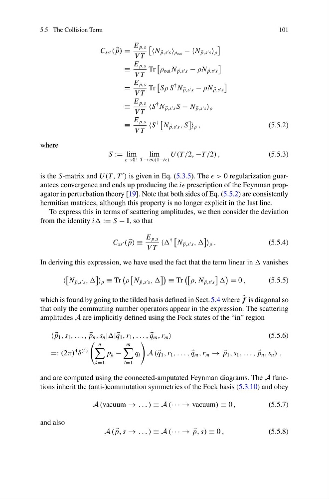
) is given in Eq. (5.3.5). The > 0 regularization guarantees convergence and ends up producing the i prescription of the Feynman propagator in perturbation theory [19]. Note that both sides of Eq. (5.5.2) are consistently
hermitian matrices, although this property is no longer explicit in the last line.
To express this in terms of scattering amplitudes, we then consider the deviation
from the identity i := S − I, so that
C ss (
p) ≡
E p,s
V T
†
N
p,s s , ,
ρ .
(5.5.4)
In deriving this expression, we have used the fact that the term linear in vanishes
N
p,s s , ,
ρ ≡ Tr
ρ
N
p,s s , ,
≡ Tr
ρ, N
p,s s
= 0 ,
(5.5.5)
which is found by going to the tilded basis defined in Sect. 5.4 where ˜ f is diagonal so
that only the commuting number operators appear in the expression. The scattering
amplitudes A are implicitly defined using the Fock states of the “in” region
p 1 , s 1 , . . . ,
p n , s n ||| q 1 , r 1 , . . . ,
q m , r m
(5.5.6)
=: (2π)
4
δ
(4)
n
k=1
p k −
m
l=1
q l
A ( q 1 , r 1 , . . . ,
q m , r m → →
p 1 , s 1 , . . . ,
p n , s n ) ,
and are computed using the connected-amputated Feynman diagrams. The A functions inherit the (anti-)commutation symmetries of the Fock basis (5.3.10) and obey
A (vacuum → . . . ) ≡ A (· · · → vacuum) ≡ 0 ,
(5.5.7)
and also
A (
p, s → . . . ) ≡ A (· · · → →
p, s) ≡ 0 ,
(5.5.8)
101
C ss (
p) =
E p,s
V T
N
p,s s ρ out − −N
p,s s ρ
≡
E p,s
V T
Tr
ρ out N
p,s s − ρN
p,s s
=
E p,s
V T
Tr
Sρ S
† N
p,s s − ρN
p,s s
≡
E p,s
V T
S
† N
p,s s S − N
p,s s ρ
≡
E p,s
V T
S
†
N
p,s s , S
ρ ,
(5.5.2)
where
S := lim
→0 +
lim
T →∞(1−i)
U (T /2, −T /2) ,
(5.5.3)
is the S-matrix and U (T, T
) is given in Eq. (5.3.5). The > 0 regularization guarantees convergence and ends up producing the i prescription of the Feynman propagator in perturbation theory [19]. Note that both sides of Eq. (5.5.2) are consistently
hermitian matrices, although this property is no longer explicit in the last line.
To express this in terms of scattering amplitudes, we then consider the deviation
from the identity i := S − I, so that
C ss (
p) ≡
E p,s
V T
†
N
p,s s , ,
ρ .
(5.5.4)
In deriving this expression, we have used the fact that the term linear in vanishes
N
p,s s , ,
ρ ≡ Tr
ρ
N
p,s s , ,
≡ Tr
ρ, N
p,s s
= 0 ,
(5.5.5)
which is found by going to the tilded basis defined in Sect. 5.4 where ˜ f is diagonal so
that only the commuting number operators appear in the expression. The scattering
amplitudes A are implicitly defined using the Fock states of the “in” region
p 1 , s 1 , . . . ,
p n , s n ||| q 1 , r 1 , . . . ,
q m , r m
(5.5.6)
=: (2π)
4
δ
(4)
n
k=1
p k −
m
l=1
q l
A ( q 1 , r 1 , . . . ,
q m , r m → →
p 1 , s 1 , . . . ,
p n , s n ) ,
and are computed using the connected-amputated Feynman diagrams. The A functions inherit the (anti-)commutation symmetries of the Fock basis (5.3.10) and obey
A (vacuum → . . . ) ≡ A (· · · → vacuum) ≡ 0 ,
(5.5.7)
and also
A (
p, s → . . . ) ≡ A (· · · → →
p, s) ≡ 0 ,
(5.5.8)