

5.4 Expressing ρ and the Entropy Current in Terms of f ss
97
that functional. It is therefore independent of w ss
δs(x)
δw ss (x,
p)
≡ 0 ,
(5.4.10)
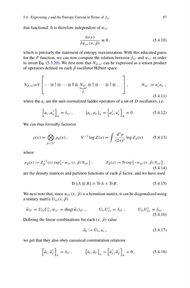
which is precisely the statement of entropy maximization. With this educated guess
for the F function, we can now compute the relation between f ss and w ss in order
to invert Eq. (5.3.20). We first note that N
p,ss can be expressed as a tensor product
of operators defined on each
p oscillator Hilbert space
N
p,ss =V
⎡
⎢
⎣· · · ⊗ I ⊗ · · · ⊗ I ⊗ N ss
p
⊗ I ⊗ · · · ⊗ I ⊗ . . .
⎤
⎥
⎦ ,
N ss := a
†
s a s ,
(5.4.11)
where the a s are the unit-normalized ladder operators of a set of D oscillators, i.e.
a s , a
†
s
±
= δ ss ,
[a s , a s ] ± =
a
†
s , a
†
s
±
= 0 .
(5.4.12)
We can thus formally factorize
ρ(x) =
p ∈ R 3
ρ
p (x) ,
V
−1 log Z (x) =
d
3 p
(2π) 3 log Z
p (x)
(5.4.13)
where
ρ
p (x) := Z
−1
p
(x) exp
−w ss (x,
p) N ss
,
Z
p (x) := Tr exp
−w ss (x,
p) N ss
,
(5.4.14)
are the density matrices and partition functions of each
p factor, and we have used
Tr [A ⊗ B] ≡ Tr A × Tr B .
(5.4.15)
We next note that, since w ss (x,
p) is a hermitian matrix, it can be diagonalized using
a unitary matrix U ˜
ss (x,
p)
˜
w ˜
s ˜
s = U ˜
ss U
∗
˜
s s w ss = diag( ˜
w ˜
s ) ˜
s ˜
s ,
U ˜
ss U
∗
˜
s s = δ ˜
s ˜
s ,
U ˜
ss U
∗
˜
ss = δ ss .
(5.4.16)
Defining the linear combinations for each (x,
p) value
˜
a ˜
s := U ˜
ss a s ,
(5.4.17)
we get that they also obey canonical commutation relations
˜
a ˜
s , ˜
a
†
˜
s
±
= δ ˜
s ˜
s ,
˜
a ˜
s , ˜
a ˜
s
±
=
˜
a
†
˜
s , ˜
a
†
˜
s
±
= 0 ,
(5.4.18)
97
that functional. It is therefore independent of w ss
δs(x)
δw ss (x,
p)
≡ 0 ,
(5.4.10)
which is precisely the statement of entropy maximization. With this educated guess
for the F function, we can now compute the relation between f ss and w ss in order
to invert Eq. (5.3.20). We first note that N
p,ss can be expressed as a tensor product
of operators defined on each
p oscillator Hilbert space
N
p,ss =V
⎡
⎢
⎣· · · ⊗ I ⊗ · · · ⊗ I ⊗ N ss
p
⊗ I ⊗ · · · ⊗ I ⊗ . . .
⎤
⎥
⎦ ,
N ss := a
†
s a s ,
(5.4.11)
where the a s are the unit-normalized ladder operators of a set of D oscillators, i.e.
a s , a
†
s
±
= δ ss ,
[a s , a s ] ± =
a
†
s , a
†
s
±
= 0 .
(5.4.12)
We can thus formally factorize
ρ(x) =
p ∈ R 3
ρ
p (x) ,
V
−1 log Z (x) =
d
3 p
(2π) 3 log Z
p (x)
(5.4.13)
where
ρ
p (x) := Z
−1
p
(x) exp
−w ss (x,
p) N ss
,
Z
p (x) := Tr exp
−w ss (x,
p) N ss
,
(5.4.14)
are the density matrices and partition functions of each
p factor, and we have used
Tr [A ⊗ B] ≡ Tr A × Tr B .
(5.4.15)
We next note that, since w ss (x,
p) is a hermitian matrix, it can be diagonalized using
a unitary matrix U ˜
ss (x,
p)
˜
w ˜
s ˜
s = U ˜
ss U
∗
˜
s s w ss = diag( ˜
w ˜
s ) ˜
s ˜
s ,
U ˜
ss U
∗
˜
s s = δ ˜
s ˜
s ,
U ˜
ss U
∗
˜
ss = δ ss .
(5.4.16)
Defining the linear combinations for each (x,
p) value
˜
a ˜
s := U ˜
ss a s ,
(5.4.17)
we get that they also obey canonical commutation relations
˜
a ˜
s , ˜
a
†
˜
s
±
= δ ˜
s ˜
s ,
˜
a ˜
s , ˜
a ˜
s
±
=
˜
a
†
˜
s , ˜
a
†
˜
s
±
= 0 ,
(5.4.18)