

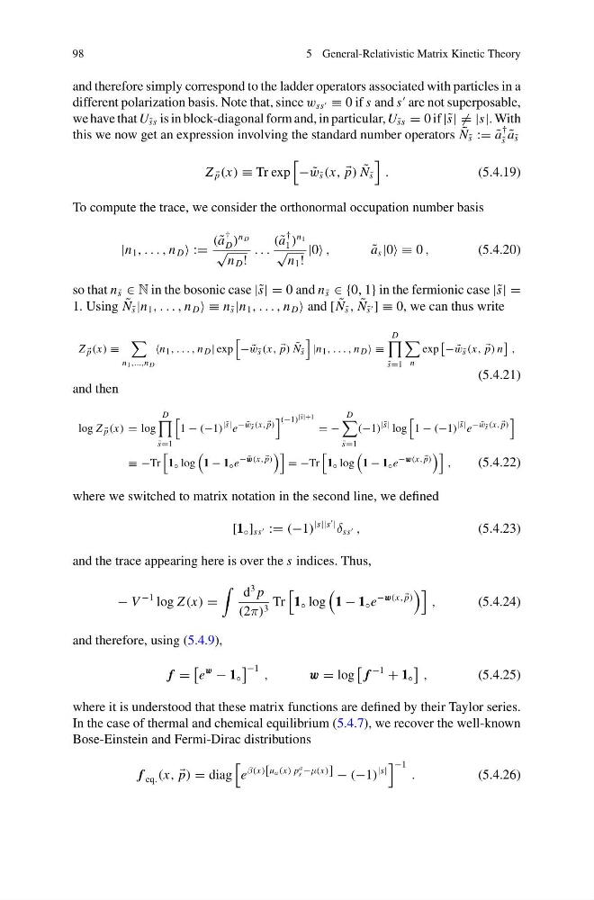
98
5 General-Relativistic Matrix Kinetic Theory
and therefore simply correspond to the ladder operators associated with particles in a
different polarization basis. Note that, since w ss ≡ 0 if s and s
are not superposable,
we have that U ˜
ss is in block-diagonal form and, in particular, U ˜
ss = 0 if |˜ s| = |s|. With
this we now get an expression involving the standard number operators ˜
N ˜
s := ˜
a
†
˜
s ˜
a ˜
s
Z
p (x) ≡ Tr exp
− ˜
w ˜
s (x,
p) ˜
N ˜
s
.
(5.4.19)
To compute the trace, we consider the orthonormal occupation number basis
|n 1 , . . . , n D :=
( ˜
a
†
D )
n D
√
n D !
. . .
( ˜
a
†
1 )
n 1
√
n 1 !
|0 ,
˜
a s |0 ≡ 0 ,
(5.4.20)
so that n ˜
s ∈ N in the bosonic case |˜ s| = 0 and n ˜
s ∈ {0, 1} in the fermionic case |˜ s| =
1. Using ˜
N ˜
s |n 1 , . . . , n D ≡ n ˜
s |n 1 , . . . , n D and [ ˜
N ˜
s , ˜
N ˜
s ] ≡ 0, we can thus write
Z
p (x) ≡
n1,...,n D
n 1 , . . . , n D | exp
− ˜
w ˜
s (x,
p) ˜
N ˜
s
|n 1 , . . . , n D ≡
D
˜
s=1
n
exp
− ˜
w ˜
s (x,
p) n
,
(5.4.21)
and then
log Z
p (x) = log
D
˜
s=1
1 − (−1)
|˜ s| e
− ˜
w ˜
s (x,
p)
(−1) |˜ s|+1
= −
D
˜
s=1
(−1)
|˜ s| log
1 − (−1)
|˜ s| e
− ˜
w ˜
s (x,
p)
≡ −Tr
1 ◦ log
1 − 1 ◦ e
− ˜
w(x,
p)
= −Tr
1 ◦ log
1 − 1 ◦ e
−w(x,
p)
,
(5.4.22)
where we switched to matrix notation in the second line, we defined
[1 ◦ ] ss := (−1)
|s||s
|
δ ss ,
(5.4.23)
and the trace appearing here is over the s indices. Thus,
− V
−1 log Z (x) =
d
3 p
(2π) 3 Tr
1 ◦ log
1 − 1 ◦ e
−w(x,
p)
,
(5.4.24)
and therefore, using (5.4.9),
f =
e
w
− 1 ◦
−1 ,
w = log
f
−1
+ 1 ◦
,
(5.4.25)
where it is understood that these matrix functions are defined by their Taylor series.
In the case of thermal and chemical equilibrium (5.4.7), we recover the well-known
Bose-Einstein and Fermi-Dirac distributions
f eq. (x,
p) = diag
e
β(x)[u a (x) p
a
s −μ(x)]
− (−1)
|s|
−1 .
(5.4.26)
5 General-Relativistic Matrix Kinetic Theory
and therefore simply correspond to the ladder operators associated with particles in a
different polarization basis. Note that, since w ss ≡ 0 if s and s
are not superposable,
we have that U ˜
ss is in block-diagonal form and, in particular, U ˜
ss = 0 if |˜ s| = |s|. With
this we now get an expression involving the standard number operators ˜
N ˜
s := ˜
a
†
˜
s ˜
a ˜
s
Z
p (x) ≡ Tr exp
− ˜
w ˜
s (x,
p) ˜
N ˜
s
.
(5.4.19)
To compute the trace, we consider the orthonormal occupation number basis
|n 1 , . . . , n D :=
( ˜
a
†
D )
n D
√
n D !
. . .
( ˜
a
†
1 )
n 1
√
n 1 !
|0 ,
˜
a s |0 ≡ 0 ,
(5.4.20)
so that n ˜
s ∈ N in the bosonic case |˜ s| = 0 and n ˜
s ∈ {0, 1} in the fermionic case |˜ s| =
1. Using ˜
N ˜
s |n 1 , . . . , n D ≡ n ˜
s |n 1 , . . . , n D and [ ˜
N ˜
s , ˜
N ˜
s ] ≡ 0, we can thus write
Z
p (x) ≡
n1,...,n D
n 1 , . . . , n D | exp
− ˜
w ˜
s (x,
p) ˜
N ˜
s
|n 1 , . . . , n D ≡
D
˜
s=1
n
exp
− ˜
w ˜
s (x,
p) n
,
(5.4.21)
and then
log Z
p (x) = log
D
˜
s=1
1 − (−1)
|˜ s| e
− ˜
w ˜
s (x,
p)
(−1) |˜ s|+1
= −
D
˜
s=1
(−1)
|˜ s| log
1 − (−1)
|˜ s| e
− ˜
w ˜
s (x,
p)
≡ −Tr
1 ◦ log
1 − 1 ◦ e
− ˜
w(x,
p)
= −Tr
1 ◦ log
1 − 1 ◦ e
−w(x,
p)
,
(5.4.22)
where we switched to matrix notation in the second line, we defined
[1 ◦ ] ss := (−1)
|s||s
|
δ ss ,
(5.4.23)
and the trace appearing here is over the s indices. Thus,
− V
−1 log Z (x) =
d
3 p
(2π) 3 Tr
1 ◦ log
1 − 1 ◦ e
−w(x,
p)
,
(5.4.24)
and therefore, using (5.4.9),
f =
e
w
− 1 ◦
−1 ,
w = log
f
−1
+ 1 ◦
,
(5.4.25)
where it is understood that these matrix functions are defined by their Taylor series.
In the case of thermal and chemical equilibrium (5.4.7), we recover the well-known
Bose-Einstein and Fermi-Dirac distributions
f eq. (x,
p) = diag
e
β(x)[u a (x) p
a
s −μ(x)]
− (−1)
|s|
−1 .
(5.4.26)