

3 Bichromatic Control of Free Electron Wave Packets
65
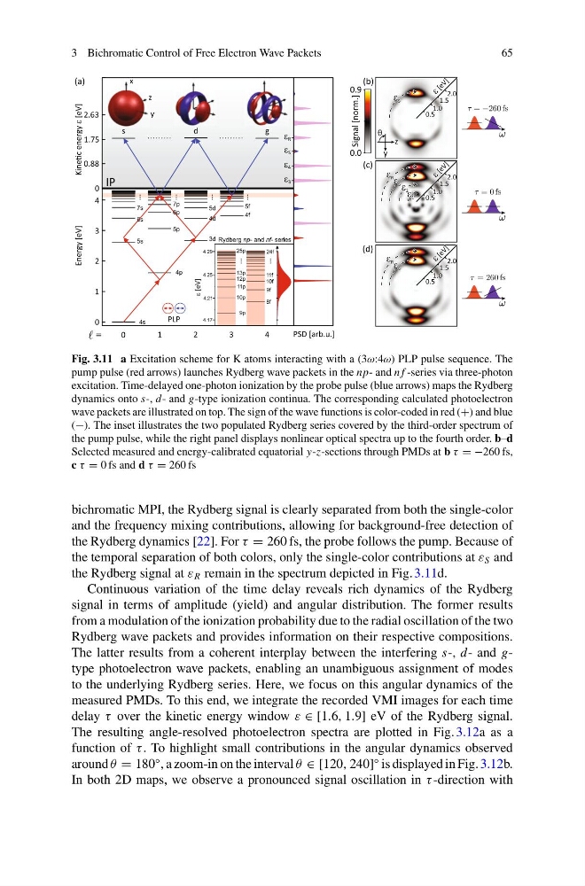
Fig. 3.11 a Excitation scheme for K atoms interacting with a (3ω:4ω) PLP pulse sequence. The
pump pulse (red arrows) launches Rydberg wave packets in the np- and n f -series via three-photon
excitation. Time-delayed one-photon ionization by the probe pulse (blue arrows) maps the Rydberg
dynamics onto s-, d- and g-type ionization continua. The corresponding calculated photoelectron
wave packets are illustrated on top. The sign of the wave functions is color-coded in red (+) and blue
(−). The inset illustrates the two populated Rydberg series covered by the third-order spectrum of
the pump pulse, while the right panel displays nonlinear optical spectra up to the fourth order. b–d
Selected measured and energy-calibrated equatorial y-z-sections through PMDs at b τ = −260 fs,
c τ = 0 fs and d τ = 260 fs
bichromatic MPI, the Rydberg signal is clearly separated from both the single-color
and the frequency mixing contributions, allowing for background-free detection of
the Rydberg dynamics [22]. For τ = 260 fs, the probe follows the pump. Because of
the temporal separation of both colors, only the single-color contributions at ε S and
the Rydberg signal at ε R remain in the spectrum depicted in Fig. 3.11d.
Continuous variation of the time delay reveals rich dynamics of the Rydberg
signal in terms of amplitude (yield) and angular distribution. The former results
from a modulation of the ionization probability due to the radial oscillation of the two
Rydberg wave packets and provides information on their respective compositions.
The latter results from a coherent interplay between the interfering s-, d- and gtype photoelectron wave packets, enabling an unambiguous assignment of modes
to the underlying Rydberg series. Here, we focus on this angular dynamics of the
measured PMDs. To this end, we integrate the recorded VMI images for each time
delay τ over the kinetic energy window ε ∈ [1.6, 1.9] eV of the Rydberg signal.
The resulting angle-resolved photoelectron spectra are plotted in Fig. 3.12a as a
function of τ . To highlight small contributions in the angular dynamics observed
around θ = 180
◦ , a zoom-in on the interval θ ∈ [120, 240]
◦ is displayed in Fig. 3.12b.
In both 2D maps, we observe a pronounced signal oscillation in τ -direction with
65
Fig. 3.11 a Excitation scheme for K atoms interacting with a (3ω:4ω) PLP pulse sequence. The
pump pulse (red arrows) launches Rydberg wave packets in the np- and n f -series via three-photon
excitation. Time-delayed one-photon ionization by the probe pulse (blue arrows) maps the Rydberg
dynamics onto s-, d- and g-type ionization continua. The corresponding calculated photoelectron
wave packets are illustrated on top. The sign of the wave functions is color-coded in red (+) and blue
(−). The inset illustrates the two populated Rydberg series covered by the third-order spectrum of
the pump pulse, while the right panel displays nonlinear optical spectra up to the fourth order. b–d
Selected measured and energy-calibrated equatorial y-z-sections through PMDs at b τ = −260 fs,
c τ = 0 fs and d τ = 260 fs
bichromatic MPI, the Rydberg signal is clearly separated from both the single-color
and the frequency mixing contributions, allowing for background-free detection of
the Rydberg dynamics [22]. For τ = 260 fs, the probe follows the pump. Because of
the temporal separation of both colors, only the single-color contributions at ε S and
the Rydberg signal at ε R remain in the spectrum depicted in Fig. 3.11d.
Continuous variation of the time delay reveals rich dynamics of the Rydberg
signal in terms of amplitude (yield) and angular distribution. The former results
from a modulation of the ionization probability due to the radial oscillation of the two
Rydberg wave packets and provides information on their respective compositions.
The latter results from a coherent interplay between the interfering s-, d- and gtype photoelectron wave packets, enabling an unambiguous assignment of modes
to the underlying Rydberg series. Here, we focus on this angular dynamics of the
measured PMDs. To this end, we integrate the recorded VMI images for each time
delay τ over the kinetic energy window ε ∈ [1.6, 1.9] eV of the Rydberg signal.
The resulting angle-resolved photoelectron spectra are plotted in Fig. 3.12a as a
function of τ . To highlight small contributions in the angular dynamics observed
around θ = 180
◦ , a zoom-in on the interval θ ∈ [120, 240]
◦ is displayed in Fig. 3.12b.
In both 2D maps, we observe a pronounced signal oscillation in τ -direction with