

170
M. F. Ciappina et al.
dc 16
dt
= c 15 w(ν 15 , 0, 0; t) − 2c 16 w(ν 16 , 0, 0; t),
(B27)
dc 17
dt
= 2c 16 w(ν 16 , 0, 0; t) − c 17 w(ν 17 , 0, 0; t),
(B28)
dc 18
dt
= c 17 w(ν 17 , 0, 0; t).
(B29)
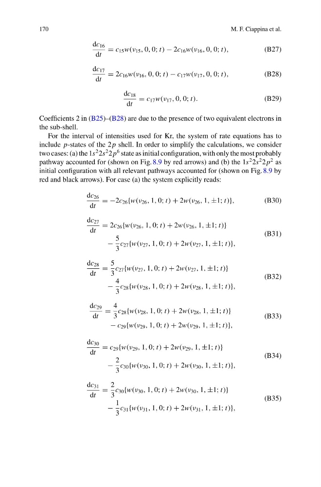
Coefficients 2 in (B25)–(B28) are due to the presence of two equivalent electrons in
the sub-shell.
For the interval of intensities used for Kr, the system of rate equations has to
include p-states of the 2 p shell. In order to simplify the calculations, we consider
two cases: (a) the 1s
2 2s
2 2 p
6 state as initial configuration, with only the most probably
pathway accounted for (shown on Fig. 8.9 by red arrows) and (b) the 1s
2 2s
2 2 p
2 as
initial configuration with all relevant pathways accounted for (shown on Fig. 8.9 by
red and black arrows). For case (a) the system explicitly reads:
dc 26
dt
= −2c 26 {w(ν 26 , 1, 0; t) + 2w(ν 26 , 1, ±1; t)},
(B30)
dc 27
dt
= 2c 26 {w(ν 26 , 1, 0; t) + 2w(ν 26 , 1, ±1; t)}
−
5
3
c 27 {w(ν 27 , 1, 0; t) + 2w(ν 27 , 1, ±1; t)},
(B31)
dc 28
dt
=
5
3
c 27 {w(ν 27 , 1, 0; t) + 2w(ν 27 , 1, ±1; t)}
−
4
3
c 28 {w(ν 28 , 1, 0; t) + 2w(ν 28 , 1, ±1; t)},
(B32)
dc 29
dt
=
4
3
c 28 {w(ν 28 , 1, 0; t) + 2w(ν 28 , 1, ±1; t)}
− c 29 {w(ν 29 , 1, 0; t) + 2w(ν 29 , 1, ±1; t)},
(B33)
dc 30
dt
= c 29 {w(ν 29 , 1, 0; t) + 2w(ν 29 , 1, ±1; t)}
−
2
3
c 30 {w(ν 30 , 1, 0; t) + 2w(ν 30 , 1, ±1; t)},
(B34)
dc 31
dt
=
2
3
c 30 {w(ν 30 , 1, 0; t) + 2w(ν 30 , 1, ±1; t)}
−
1
3
c 31 {w(ν 31 , 1, 0; t) + 2w(ν 31 , 1, ±1; t)},
(B35)
M. F. Ciappina et al.
dc 16
dt
= c 15 w(ν 15 , 0, 0; t) − 2c 16 w(ν 16 , 0, 0; t),
(B27)
dc 17
dt
= 2c 16 w(ν 16 , 0, 0; t) − c 17 w(ν 17 , 0, 0; t),
(B28)
dc 18
dt
= c 17 w(ν 17 , 0, 0; t).
(B29)
Coefficients 2 in (B25)–(B28) are due to the presence of two equivalent electrons in
the sub-shell.
For the interval of intensities used for Kr, the system of rate equations has to
include p-states of the 2 p shell. In order to simplify the calculations, we consider
two cases: (a) the 1s
2 2s
2 2 p
6 state as initial configuration, with only the most probably
pathway accounted for (shown on Fig. 8.9 by red arrows) and (b) the 1s
2 2s
2 2 p
2 as
initial configuration with all relevant pathways accounted for (shown on Fig. 8.9 by
red and black arrows). For case (a) the system explicitly reads:
dc 26
dt
= −2c 26 {w(ν 26 , 1, 0; t) + 2w(ν 26 , 1, ±1; t)},
(B30)
dc 27
dt
= 2c 26 {w(ν 26 , 1, 0; t) + 2w(ν 26 , 1, ±1; t)}
−
5
3
c 27 {w(ν 27 , 1, 0; t) + 2w(ν 27 , 1, ±1; t)},
(B31)
dc 28
dt
=
5
3
c 27 {w(ν 27 , 1, 0; t) + 2w(ν 27 , 1, ±1; t)}
−
4
3
c 28 {w(ν 28 , 1, 0; t) + 2w(ν 28 , 1, ±1; t)},
(B32)
dc 29
dt
=
4
3
c 28 {w(ν 28 , 1, 0; t) + 2w(ν 28 , 1, ±1; t)}
− c 29 {w(ν 29 , 1, 0; t) + 2w(ν 29 , 1, ±1; t)},
(B33)
dc 30
dt
= c 29 {w(ν 29 , 1, 0; t) + 2w(ν 29 , 1, ±1; t)}
−
2
3
c 30 {w(ν 30 , 1, 0; t) + 2w(ν 30 , 1, ±1; t)},
(B34)
dc 31
dt
=
2
3
c 30 {w(ν 30 , 1, 0; t) + 2w(ν 30 , 1, ±1; t)}
−
1
3
c 31 {w(ν 31 , 1, 0; t) + 2w(ν 31 , 1, ±1; t)},
(B35)