

8 Towards Laser Intensity Calibration Using High-Field Ionization
159
8.2.4 Effect of the Intensity Space Distribution
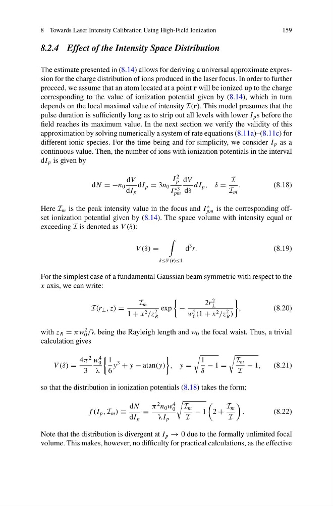
The estimate presented in (8.14) allows for deriving a universal approximate expression for the charge distribution of ions produced in the laser focus. In order to further
proceed, we assume that an atom located at a point r will be ionized up to the charge
corresponding to the value of ionization potential given by (8.14), which in turn
depends on the local maximal value of intensity I(r). This model presumes that the
pulse duration is sufficiently long as to strip out all levels with lower I p s before the
field reaches its maximum value. In the next section we verify the validity of this
approximation by solving numerically a system of rate equations (8.11a)–(8.11c) for
different ionic species. For the time being and for simplicity, we consider I p as a
continuous value. Then, the number of ions with ionization potentials in the interval
dI p is given by
dN = −n 0
dV
dI p
dI p = 3n 0
I
2
p
I ∗3
pm
dV
dδ
d I p , δ =
I
I m
.
(8.18)
Here I m is the peak intensity value in the focus and I
∗
pm is the corresponding offset ionization potential given by (8.14). The space volume with intensity equal or
exceeding I is denoted as V (δ):
V (δ) =
δ≤δ (r)≤1
d
3 r.
(8.19)
For the simplest case of a fundamental Gaussian beam symmetric with respect to the
x axis, we can write:
I(r ⊥ , z) =
I m
1 + x 2 /z
2
R
exp
−
2r
2
⊥
w
2
0 (1 + x 2 /z
2
R )
,
(8.20)
with z R = π w
2
0 /λ being the Rayleigh length and w 0 the focal waist. Thus, a trivial
calculation gives
V (δ) =
4π
2
3
w
4
0
λ
1
6
y
3
+ y − atan(y)
, y =
1
δ
− 1 =
I m
I
− 1,
(8.21)
so that the distribution in ionization potentials (8.18) takes the form:
f (I p , I m ) ≡
dN
dI p
=
π
2 n 0 w
4
0
λI p
I m
I
− 1
2 +
I m
I
.
(8.22)
Note that the distribution is divergent at I p → 0 due to the formally unlimited focal
volume. This makes, however, no difficulty for practical calculations, as the effective
159
8.2.4 Effect of the Intensity Space Distribution
The estimate presented in (8.14) allows for deriving a universal approximate expression for the charge distribution of ions produced in the laser focus. In order to further
proceed, we assume that an atom located at a point r will be ionized up to the charge
corresponding to the value of ionization potential given by (8.14), which in turn
depends on the local maximal value of intensity I(r). This model presumes that the
pulse duration is sufficiently long as to strip out all levels with lower I p s before the
field reaches its maximum value. In the next section we verify the validity of this
approximation by solving numerically a system of rate equations (8.11a)–(8.11c) for
different ionic species. For the time being and for simplicity, we consider I p as a
continuous value. Then, the number of ions with ionization potentials in the interval
dI p is given by
dN = −n 0
dV
dI p
dI p = 3n 0
I
2
p
I ∗3
pm
dV
dδ
d I p , δ =
I
I m
.
(8.18)
Here I m is the peak intensity value in the focus and I
∗
pm is the corresponding offset ionization potential given by (8.14). The space volume with intensity equal or
exceeding I is denoted as V (δ):
V (δ) =
δ≤δ (r)≤1
d
3 r.
(8.19)
For the simplest case of a fundamental Gaussian beam symmetric with respect to the
x axis, we can write:
I(r ⊥ , z) =
I m
1 + x 2 /z
2
R
exp
−
2r
2
⊥
w
2
0 (1 + x 2 /z
2
R )
,
(8.20)
with z R = π w
2
0 /λ being the Rayleigh length and w 0 the focal waist. Thus, a trivial
calculation gives
V (δ) =
4π
2
3
w
4
0
λ
1
6
y
3
+ y − atan(y)
, y =
1
δ
− 1 =
I m
I
− 1,
(8.21)
so that the distribution in ionization potentials (8.18) takes the form:
f (I p , I m ) ≡
dN
dI p
=
π
2 n 0 w
4
0
λI p
I m
I
− 1
2 +
I m
I
.
(8.22)
Note that the distribution is divergent at I p → 0 due to the formally unlimited focal
volume. This makes, however, no difficulty for practical calculations, as the effective