

162
M. Kiran Raj and S. Chakraborty
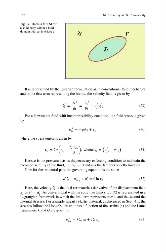
Fig. 12 Domain for FSI for
a solid body within a fluid
domain with an interface Γ
It is represented by the Eulerian formulation as in conventional fluid mechanics
and in the first term representing the inertia, the velocity field is given by
˙
v
f
i =
dv
f
i
dt
=
∂v
f
i
∂t
+ v
f
j v
f
i, j
(29)
For a Newtonian fluid with incompressibility condition, the fluid stress is given
by
σ
f
i j = −pδ i j + τ i j
(30)
where the stress tensor is given by
τ i j = 2μ
e i j −
δ i j e kk
3
, where e i j =
v
f
j,i + v
f
i, j
(31)
Here, p is the pressure acts as the necessary enforcing condition to maintain the
incompressibility of the fluid, i.e., v
f
i,i = 0 and δ is the Kronecker delta function.
Now for the structural part, the governing equation is the same
ρ
s
˙
v i − σ
s
i j, j + b
s
i = 0 in χ s
(32)
Here, the velocity ˙
v
s
i is the total (or material) derivative of the displacement field
u
s
i or v
s
i = ˙
u
s
i . As conventional with the solid mechanics, Eq. 32 is represented in a
Lagrangian framework in which the first term represents inertia and the second the
internal stresses. For a simple linearly elastic material, as discussed in Sect. 4.1, the
stresses follow the Hooke’s law and thus a function of the strains () and the Lamé
parameters λ and G are given by
σ
s
i, j = λδ i j ll + 2G i j
(33)
M. Kiran Raj and S. Chakraborty
Fig. 12 Domain for FSI for
a solid body within a fluid
domain with an interface Γ
It is represented by the Eulerian formulation as in conventional fluid mechanics
and in the first term representing the inertia, the velocity field is given by
˙
v
f
i =
dv
f
i
dt
=
∂v
f
i
∂t
+ v
f
j v
f
i, j
(29)
For a Newtonian fluid with incompressibility condition, the fluid stress is given
by
σ
f
i j = −pδ i j + τ i j
(30)
where the stress tensor is given by
τ i j = 2μ
e i j −
δ i j e kk
3
, where e i j =
v
f
j,i + v
f
i, j
(31)
Here, p is the pressure acts as the necessary enforcing condition to maintain the
incompressibility of the fluid, i.e., v
f
i,i = 0 and δ is the Kronecker delta function.
Now for the structural part, the governing equation is the same
ρ
s
˙
v i − σ
s
i j, j + b
s
i = 0 in χ s
(32)
Here, the velocity ˙
v
s
i is the total (or material) derivative of the displacement field
u
s
i or v
s
i = ˙
u
s
i . As conventional with the solid mechanics, Eq. 32 is represented in a
Lagrangian framework in which the first term represents inertia and the second the
internal stresses. For a simple linearly elastic material, as discussed in Sect. 4.1, the
stresses follow the Hooke’s law and thus a function of the strains () and the Lamé
parameters λ and G are given by
σ
s
i, j = λδ i j ll + 2G i j
(33)