

Fluid Dynamics in Deformable Microchannels
155
4.1 Cylindrical Channel [2]
Figure 7 shows the schematic of the microchannel of radius R in a rectangular block
of dimensions L, W, and H. Note that our configuration is different from a thinwalled tube configuration for which there is a well-established relationship for the
deformation. The mechanical equilibrium equations are given by
∇ · σ = 0,
(8)
where σ is the stress tensor. As the channel is axisymmetric and slender, the radial
component of the mechanical equilibrium equations reduces to
1
r
∂
∂r
(r σ rr ) −
σ θθ
r
= 0,
(9)
where σ rr and σ θθ are the normal components of the stress tensor in the radial
and the angular directions, respectively. Note that the term involving σ r z scales
out because we assume zero axial displacement and because of the smallness of
the radial displacement compared to the characteristic axial length scale. These
reductions are equivalent to the lubrication approximation for fluid flow through
narrow confinements. For the solid material, we use linear, elastic, isotropic behavior
given by
σ = λ(∇ · α)I + 2G
1
2
(∇α) + (∇α)
T
(10)
where λ and G are the Lamé parameters, I is the identity tensor, and α is the displacement vector in the cylindrical coordinates given by α =
α r α θ α z
T . Using the same
considerations that were used to reduce the mechanical equilibrium equations, we
obtain
σ rr = λ
1
r
∂
∂r
(r α r ) + 2G
∂α r
∂r
(11)
σ θθ = λ
1
r
∂
∂r
(r α r ) + 2G
α r
r
.
(12)
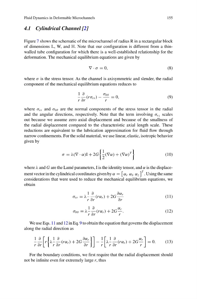
We use Eqs. 11 and 12 in Eq. 9 to obtain the equation that governs the displacement
along the radial direction as
1
r
∂
∂r
r
λ
1
r
∂
∂r
(r α r ) + 2G
∂α r
∂r
−
1
r
λ
1
r
∂
∂r
(r α r ) + 2G
α r
r
= 0.
(13)
For the boundary conditions, we first require that the radial displacement should
not be infinite even for extremely large r, thus
155
4.1 Cylindrical Channel [2]
Figure 7 shows the schematic of the microchannel of radius R in a rectangular block
of dimensions L, W, and H. Note that our configuration is different from a thinwalled tube configuration for which there is a well-established relationship for the
deformation. The mechanical equilibrium equations are given by
∇ · σ = 0,
(8)
where σ is the stress tensor. As the channel is axisymmetric and slender, the radial
component of the mechanical equilibrium equations reduces to
1
r
∂
∂r
(r σ rr ) −
σ θθ
r
= 0,
(9)
where σ rr and σ θθ are the normal components of the stress tensor in the radial
and the angular directions, respectively. Note that the term involving σ r z scales
out because we assume zero axial displacement and because of the smallness of
the radial displacement compared to the characteristic axial length scale. These
reductions are equivalent to the lubrication approximation for fluid flow through
narrow confinements. For the solid material, we use linear, elastic, isotropic behavior
given by
σ = λ(∇ · α)I + 2G
1
2
(∇α) + (∇α)
T
(10)
where λ and G are the Lamé parameters, I is the identity tensor, and α is the displacement vector in the cylindrical coordinates given by α =
α r α θ α z
T . Using the same
considerations that were used to reduce the mechanical equilibrium equations, we
obtain
σ rr = λ
1
r
∂
∂r
(r α r ) + 2G
∂α r
∂r
(11)
σ θθ = λ
1
r
∂
∂r
(r α r ) + 2G
α r
r
.
(12)
We use Eqs. 11 and 12 in Eq. 9 to obtain the equation that governs the displacement
along the radial direction as
1
r
∂
∂r
r
λ
1
r
∂
∂r
(r α r ) + 2G
∂α r
∂r
−
1
r
λ
1
r
∂
∂r
(r α r ) + 2G
α r
r
= 0.
(13)
For the boundary conditions, we first require that the radial displacement should
not be infinite even for extremely large r, thus