

126
G. Biswas and K. C. Sahu
and-cell (MAC) scheme [15], the volume-of-fluid (VoF) method [16–19], level-set
(LS) method and coupled level-set volume-of-fluid (CLSVOF) approach [20–22] are
some examples of the interface capturing technique. In some cases, hybrid methods
have been used to simulate interfacial flows. Here, we do not discuss all the methods, but in what follows, only highlight the coupled level-set and volume-of-fluid
(CLSVOF) approach.
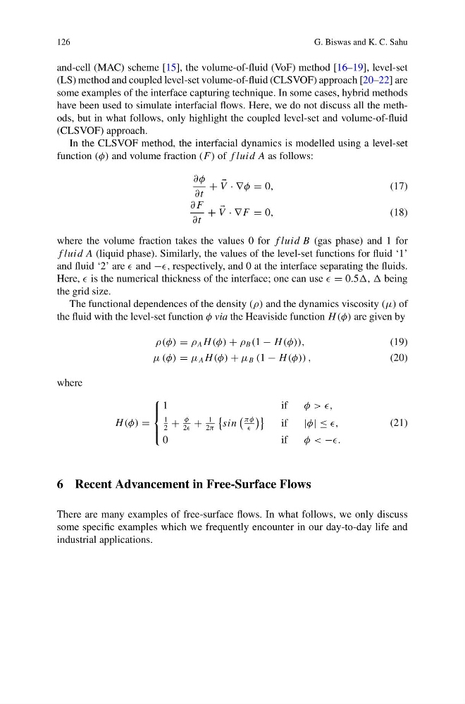
In the CLSVOF method, the interfacial dynamics is modelled using a level-set
function (φ) and volume fraction (F) of f luid A as follows:
∂φ
∂t
+
V · ∇φ = 0,
(17)
∂ F
∂t
+
V · ∇ F = 0,
(18)
where the volume fraction takes the values 0 for f luid B (gas phase) and 1 for
f luid A (liquid phase). Similarly, the values of the level-set functions for fluid ‘1’
and fluid ‘2’ are and −, respectively, and 0 at the interface separating the fluids.
Here, is the numerical thickness of the interface; one can use = 0.5, being
the grid size.
The functional dependences of the density (ρ) and the dynamics viscosity (μ) of
the fluid with the level-set function φ via the Heaviside function H (φ) are given by
ρ(φ) = ρ A H (φ) + ρ B (1 − H (φ)),
(19)
μ (φ) = μ A H (φ) + μ B (1 − H (φ)) ,
(20)
where
H (φ) =
⎧
⎪ ⎨
⎪ ⎩
1
i f
φ > >,
1
2
+
φ
2
+
1
2π
sin
πφ
if
|φ| ≤ ,
0
i f
φ < −.
(21)
6 Recent Advancement in Free-Surface Flows
There are many examples of free-surface flows. In what follows, we only discuss
some specific examples which we frequently encounter in our day-to-day life and
industrial applications.
G. Biswas and K. C. Sahu
and-cell (MAC) scheme [15], the volume-of-fluid (VoF) method [16–19], level-set
(LS) method and coupled level-set volume-of-fluid (CLSVOF) approach [20–22] are
some examples of the interface capturing technique. In some cases, hybrid methods
have been used to simulate interfacial flows. Here, we do not discuss all the methods, but in what follows, only highlight the coupled level-set and volume-of-fluid
(CLSVOF) approach.
In the CLSVOF method, the interfacial dynamics is modelled using a level-set
function (φ) and volume fraction (F) of f luid A as follows:
∂φ
∂t
+
V · ∇φ = 0,
(17)
∂ F
∂t
+
V · ∇ F = 0,
(18)
where the volume fraction takes the values 0 for f luid B (gas phase) and 1 for
f luid A (liquid phase). Similarly, the values of the level-set functions for fluid ‘1’
and fluid ‘2’ are and −, respectively, and 0 at the interface separating the fluids.
Here, is the numerical thickness of the interface; one can use = 0.5, being
the grid size.
The functional dependences of the density (ρ) and the dynamics viscosity (μ) of
the fluid with the level-set function φ via the Heaviside function H (φ) are given by
ρ(φ) = ρ A H (φ) + ρ B (1 − H (φ)),
(19)
μ (φ) = μ A H (φ) + μ B (1 − H (φ)) ,
(20)
where
H (φ) =
⎧
⎪ ⎨
⎪ ⎩
1
i f
φ > >,
1
2
+
φ
2
+
1
2π
sin
πφ
if
|φ| ≤ ,
0
i f
φ < −.
(21)
6 Recent Advancement in Free-Surface Flows
There are many examples of free-surface flows. In what follows, we only discuss
some specific examples which we frequently encounter in our day-to-day life and
industrial applications.