

118
A. K. Misra and S. Cohen
where
B = [α, B 1 , B 2 , . . . , B k ]
T
(42)
and the elements of matrices M
B and K
B are given by
M 11 B = (1 + ε 0 )
2
M p
1
0
exp[F(ξ)]ξ
2 dξ + M c
(43)
K
B
11 = (1 + ε 0 )
2
1
Λ
M p
1
0
exp[F(ξ)]ξdξ + M c
−
β
3
Λ 4
M p
1
0
exp[F(ξ)]ξ
[(1/Λ) + ξ(1 + ε 0 )] 3 dξ + M c
1
[(1/Λ) + (1 + ε 0 )] 3
(44)
M
B
i1 = M
B
1k = M p (1 + ε 0 )
1
0
exp[F(ξ)]ξφ i dξ
(45)
K
B
i1 = K
B
1k = M p
1
Λ
1
0
exp[F(ξ)]φ i dξ −
β
3
Λ 4
1
0
exp[F(ξ)]φ i
[(1/Λ) + ξ(1 + ε 0 )] 3 dξ
(46)
M
B
ik =
1
0
exp[F(ξ)]ψ i ψ k dξ
(47)
K
B
ik = π
2
(ε 0 − ε
2
0 )ik ¯
Ω
2
1
0
exp[F(ξ)]
dφ i
dξ
dφ k
dξ
dξ
+ M p
β
Λ
3
1
0
exp[F(ξ)]φ i
[(1/Λ) + ξ(1 + ε 0 )] 3 dξ −
1
0
exp[F(ξ)]φ i φ k dξ
(48)
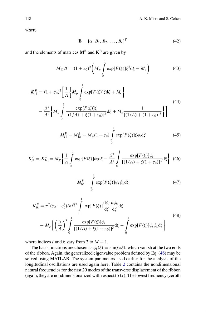
where indices i and k vary from 2 to M + 1.
The basis functions are chosen as φ i (ξ) = sin(iπξ), which vanish at the two ends
of the ribbon. Again, the generalized eigenvalue problem defined by Eq. (46) may be
solved using MATLAB. The system parameters used earlier for the analysis of the
longitudinal oscillations are used again here. Table 2 contains the nondimensional
natural frequencies for the first 20 modes of the transverse displacement of the ribbon
(again, they are nondimensionalized with respect to Ω). The lowest frequency (zeroth
A. K. Misra and S. Cohen
where
B = [α, B 1 , B 2 , . . . , B k ]
T
(42)
and the elements of matrices M
B and K
B are given by
M 11 B = (1 + ε 0 )
2
M p
1
0
exp[F(ξ)]ξ
2 dξ + M c
(43)
K
B
11 = (1 + ε 0 )
2
1
Λ
M p
1
0
exp[F(ξ)]ξdξ + M c
−
β
3
Λ 4
M p
1
0
exp[F(ξ)]ξ
[(1/Λ) + ξ(1 + ε 0 )] 3 dξ + M c
1
[(1/Λ) + (1 + ε 0 )] 3
(44)
M
B
i1 = M
B
1k = M p (1 + ε 0 )
1
0
exp[F(ξ)]ξφ i dξ
(45)
K
B
i1 = K
B
1k = M p
1
Λ
1
0
exp[F(ξ)]φ i dξ −
β
3
Λ 4
1
0
exp[F(ξ)]φ i
[(1/Λ) + ξ(1 + ε 0 )] 3 dξ
(46)
M
B
ik =
1
0
exp[F(ξ)]ψ i ψ k dξ
(47)
K
B
ik = π
2
(ε 0 − ε
2
0 )ik ¯
Ω
2
1
0
exp[F(ξ)]
dφ i
dξ
dφ k
dξ
dξ
+ M p
β
Λ
3
1
0
exp[F(ξ)]φ i
[(1/Λ) + ξ(1 + ε 0 )] 3 dξ −
1
0
exp[F(ξ)]φ i φ k dξ
(48)
where indices i and k vary from 2 to M + 1.
The basis functions are chosen as φ i (ξ) = sin(iπξ), which vanish at the two ends
of the ribbon. Again, the generalized eigenvalue problem defined by Eq. (46) may be
solved using MATLAB. The system parameters used earlier for the analysis of the
longitudinal oscillations are used again here. Table 2 contains the nondimensional
natural frequencies for the first 20 modes of the transverse displacement of the ribbon
(again, they are nondimensionalized with respect to Ω). The lowest frequency (zeroth