

Automated Upgraded Generalized Full-Discretization Method …
93
analysis. The approach as pioneered in [30] is not directly applicable to thin-walled
workpiece and thus needs upgrading (as done here) by the incorporation of model
order reduction for automatic computation of the reduced model matrices A and B(t)
at every computational time step of stability analysis.
4 Numerical Results and Discussion
In this section, the full computerization of thin-walled milling stability analysis and its
application to revealing the parametric effect of interpolation order on computational
precision and time are demonstrated. The generalized monodromy matrix given in
Eq. (17) is programmed in a MATLAB script which incorporates the parameters of
the milling process and the workpiece adopted from [23]. The thin-walled workpiece is a 0.17 m × 0.03 m × 0.15 m steel material of density =7.8×10
3 kgm
−3 ,
Young’s modulus E = 210 × 10
−9 Nm
−2 , and Poisson’s ratio v pr = 0.3. These geometric and material properties were used to generate the modal matrices which were
reduced with three eigenmodes. The two-tooth tool is subjected to up-milling at
radial immersion ρ = 0.25. The feed per tooth is 0.1 mm, the tangential cutting
coefficient is C t = 1.07 × 10
8 Nm
−1−γ , the force law feed exponent is γ = 0.75,
and the normal-to-tangential force ratio is χ =
40
107
.
4.1 Rate of Convergence with Order
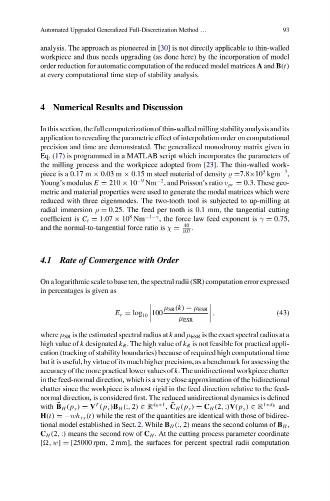
On a logarithmic scale to base ten, the spectral radii (SR) computation error expressed
in percentages is given as
E c = log 10
100
μ SR (k) − μ ESR
μ ESR
,
(43)
where μ SR is the estimated spectral radius at k and μ ESR is the exact spectral radius at a
high value of k designated k R . The high value of k R is not feasible for practical application (tracking of stability boundaries) because of required high computational time
but it is useful, by virtue of its much higher precision, as a benchmark for assessing the
accuracy of the more practical lower values of k. The unidirectional workpiece chatter
in the feed-normal direction, which is a very close approximation of the bidirectional
chatter since the workpiece is almost rigid in the feed direction relative to the feednormal direction, is considered first. The reduced unidirectional dynamics is defined
with ˜
B H ( p y ) = V
T
( p y )B H (:, 2) ∈ R
d R ×1 , ˜
C H ( p y ) = C H (2, :)V( p y ) ∈ R
1×d R and
H(t) = −wh yy (t) while the rest of the quantities are identical with those of bidirectional model established in Sect. 2. While B H (:, 2) means the second column of B H ,
C H (2, :) means the second row of C H . At the cutting process parameter coordinate
[, w] = [25000 rpm, 2 mm], the surfaces for percent spectral radii computation
93
analysis. The approach as pioneered in [30] is not directly applicable to thin-walled
workpiece and thus needs upgrading (as done here) by the incorporation of model
order reduction for automatic computation of the reduced model matrices A and B(t)
at every computational time step of stability analysis.
4 Numerical Results and Discussion
In this section, the full computerization of thin-walled milling stability analysis and its
application to revealing the parametric effect of interpolation order on computational
precision and time are demonstrated. The generalized monodromy matrix given in
Eq. (17) is programmed in a MATLAB script which incorporates the parameters of
the milling process and the workpiece adopted from [23]. The thin-walled workpiece is a 0.17 m × 0.03 m × 0.15 m steel material of density =7.8×10
3 kgm
−3 ,
Young’s modulus E = 210 × 10
−9 Nm
−2 , and Poisson’s ratio v pr = 0.3. These geometric and material properties were used to generate the modal matrices which were
reduced with three eigenmodes. The two-tooth tool is subjected to up-milling at
radial immersion ρ = 0.25. The feed per tooth is 0.1 mm, the tangential cutting
coefficient is C t = 1.07 × 10
8 Nm
−1−γ , the force law feed exponent is γ = 0.75,
and the normal-to-tangential force ratio is χ =
40
107
.
4.1 Rate of Convergence with Order
On a logarithmic scale to base ten, the spectral radii (SR) computation error expressed
in percentages is given as
E c = log 10
100
μ SR (k) − μ ESR
μ ESR
,
(43)
where μ SR is the estimated spectral radius at k and μ ESR is the exact spectral radius at a
high value of k designated k R . The high value of k R is not feasible for practical application (tracking of stability boundaries) because of required high computational time
but it is useful, by virtue of its much higher precision, as a benchmark for assessing the
accuracy of the more practical lower values of k. The unidirectional workpiece chatter
in the feed-normal direction, which is a very close approximation of the bidirectional
chatter since the workpiece is almost rigid in the feed direction relative to the feednormal direction, is considered first. The reduced unidirectional dynamics is defined
with ˜
B H ( p y ) = V
T
( p y )B H (:, 2) ∈ R
d R ×1 , ˜
C H ( p y ) = C H (2, :)V( p y ) ∈ R
1×d R and
H(t) = −wh yy (t) while the rest of the quantities are identical with those of bidirectional model established in Sect. 2. While B H (:, 2) means the second column of B H ,
C H (2, :) means the second row of C H . At the cutting process parameter coordinate
[, w] = [25000 rpm, 2 mm], the surfaces for percent spectral radii computation