

7 Intelligent and Connected Cyber-Physical Systems: A Perspective. . .
369
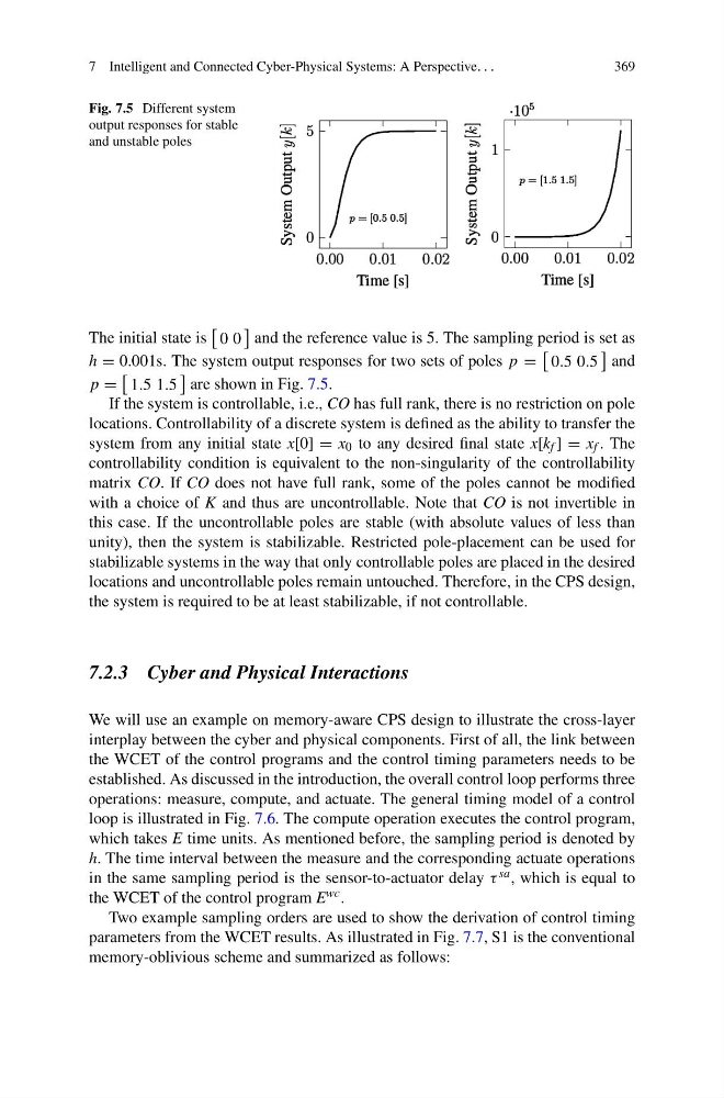
Fig. 7.5 Different system
output responses for stable
and unstable poles
The initial state is
0 0
and the reference value is 5. The sampling period is set as
h = 0.001s. The system output responses for two sets of poles p =
0.5 0.5
and
p =
1.5 1.5
are shown in Fig. 7.5.
If the system is controllable, i.e., CO has full rank, there is no restriction on pole
locations. Controllability of a discrete system is defined as the ability to transfer the
system from any initial state x[0] = x 0 to any desired final state x[k f ] = x f . The
controllability condition is equivalent to the non-singularity of the controllability
matrix CO. If CO does not have full rank, some of the poles cannot be modified
with a choice of K and thus are uncontrollable. Note that CO is not invertible in
this case. If the uncontrollable poles are stable (with absolute values of less than
unity), then the system is stabilizable. Restricted pole-placement can be used for
stabilizable systems in the way that only controllable poles are placed in the desired
locations and uncontrollable poles remain untouched. Therefore, in the CPS design,
the system is required to be at least stabilizable, if not controllable.
7.2.3 Cyber and Physical Interactions
We will use an example on memory-aware CPS design to illustrate the cross-layer
interplay between the cyber and physical components. First of all, the link between
the WCET of the control programs and the control timing parameters needs to be
established. As discussed in the introduction, the overall control loop performs three
operations: measure, compute, and actuate. The general timing model of a control
loop is illustrated in Fig. 7.6. The compute operation executes the control program,
which takes E time units. As mentioned before, the sampling period is denoted by
h. The time interval between the measure and the corresponding actuate operations
in the same sampling period is the sensor-to-actuator delay τ sa , which is equal to
the WCET of the control program E wc .
Two example sampling orders are used to show the derivation of control timing
parameters from the WCET results. As illustrated in Fig. 7.7, S1 is the conventional
memory-oblivious scheme and summarized as follows:
369
Fig. 7.5 Different system
output responses for stable
and unstable poles
The initial state is
0 0
and the reference value is 5. The sampling period is set as
h = 0.001s. The system output responses for two sets of poles p =
0.5 0.5
and
p =
1.5 1.5
are shown in Fig. 7.5.
If the system is controllable, i.e., CO has full rank, there is no restriction on pole
locations. Controllability of a discrete system is defined as the ability to transfer the
system from any initial state x[0] = x 0 to any desired final state x[k f ] = x f . The
controllability condition is equivalent to the non-singularity of the controllability
matrix CO. If CO does not have full rank, some of the poles cannot be modified
with a choice of K and thus are uncontrollable. Note that CO is not invertible in
this case. If the uncontrollable poles are stable (with absolute values of less than
unity), then the system is stabilizable. Restricted pole-placement can be used for
stabilizable systems in the way that only controllable poles are placed in the desired
locations and uncontrollable poles remain untouched. Therefore, in the CPS design,
the system is required to be at least stabilizable, if not controllable.
7.2.3 Cyber and Physical Interactions
We will use an example on memory-aware CPS design to illustrate the cross-layer
interplay between the cyber and physical components. First of all, the link between
the WCET of the control programs and the control timing parameters needs to be
established. As discussed in the introduction, the overall control loop performs three
operations: measure, compute, and actuate. The general timing model of a control
loop is illustrated in Fig. 7.6. The compute operation executes the control program,
which takes E time units. As mentioned before, the sampling period is denoted by
h. The time interval between the measure and the corresponding actuate operations
in the same sampling period is the sensor-to-actuator delay τ sa , which is equal to
the WCET of the control program E wc .
Two example sampling orders are used to show the derivation of control timing
parameters from the WCET results. As illustrated in Fig. 7.7, S1 is the conventional
memory-oblivious scheme and summarized as follows: