

368
W. Chang et al.
where K is the feedback gain and F is the feedforward gain. Clearly, the relationship
between u[k] and x[k] is linear. With this controller, the system dynamics becomes
x [k + 1] = (A d + B d K) x [k] + B d F r,
i.e., closed-loop dynamics.
Different locations of closed-loop system poles, i.e., eigenvalues of (A d + B d K),
result in different system behavior. In pole-placement, poles are placed in desired
locations (eigenvalues are set) often to fulfil various high-level goals, such as control
performance maximization and system constraints satisfaction. The desired poles p
can be decided with empirical or optimization techniques. This method is feasible
since there is freedom to choose the feedback gain K. Once pole locations are
decided, the following characteristics equation of z can be constructed with these
poles as roots:
z
n
+ γ 1 z
n−1
+ γ 2 z
n−2
+ · · · + γ n = 0.
Then the following is defined:
γ c (A d ) = A
n
d + γ 1 A
n−1
d
+ γ 2 A
n−2
d
+ · · · + γ n I .
According to Ackermann’s formula, the feedback gain used to stabilize the closedloop system is calculated as
K = [0 · · · 0 1] CO
−1 γ c (A d ) ,
where
CO =
B d A d B d · · · A
n−1
d B d
is the square controllability matrix. The static feedforward gain F used to make the
system output y[k] track the reference r is computed by
F =
1
C d (I − A d − B d K)
−1 B d
.
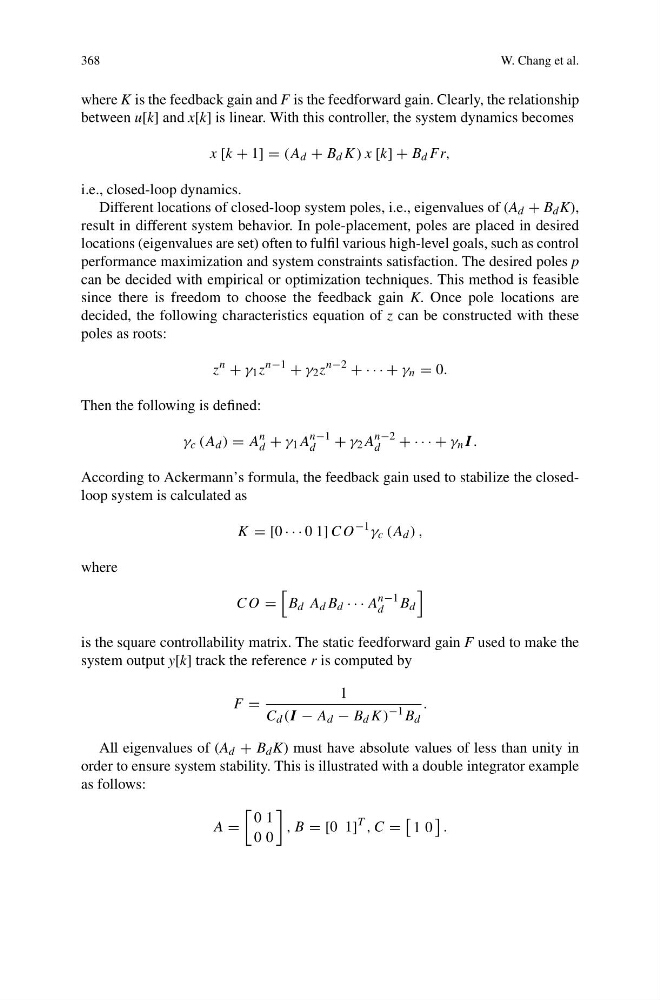
All eigenvalues of (A d + B d K) must have absolute values of less than unity in
order to ensure system stability. This is illustrated with a double integrator example
as follows:
A =
0 1
0 0
, B = [0 1]
T , C =
1 0
.
W. Chang et al.
where K is the feedback gain and F is the feedforward gain. Clearly, the relationship
between u[k] and x[k] is linear. With this controller, the system dynamics becomes
x [k + 1] = (A d + B d K) x [k] + B d F r,
i.e., closed-loop dynamics.
Different locations of closed-loop system poles, i.e., eigenvalues of (A d + B d K),
result in different system behavior. In pole-placement, poles are placed in desired
locations (eigenvalues are set) often to fulfil various high-level goals, such as control
performance maximization and system constraints satisfaction. The desired poles p
can be decided with empirical or optimization techniques. This method is feasible
since there is freedom to choose the feedback gain K. Once pole locations are
decided, the following characteristics equation of z can be constructed with these
poles as roots:
z
n
+ γ 1 z
n−1
+ γ 2 z
n−2
+ · · · + γ n = 0.
Then the following is defined:
γ c (A d ) = A
n
d + γ 1 A
n−1
d
+ γ 2 A
n−2
d
+ · · · + γ n I .
According to Ackermann’s formula, the feedback gain used to stabilize the closedloop system is calculated as
K = [0 · · · 0 1] CO
−1 γ c (A d ) ,
where
CO =
B d A d B d · · · A
n−1
d B d
is the square controllability matrix. The static feedforward gain F used to make the
system output y[k] track the reference r is computed by
F =
1
C d (I − A d − B d K)
−1 B d
.
All eigenvalues of (A d + B d K) must have absolute values of less than unity in
order to ensure system stability. This is illustrated with a double integrator example
as follows:
A =
0 1
0 0
, B = [0 1]
T , C =
1 0
.