

5 Machine Learning for IoT
285
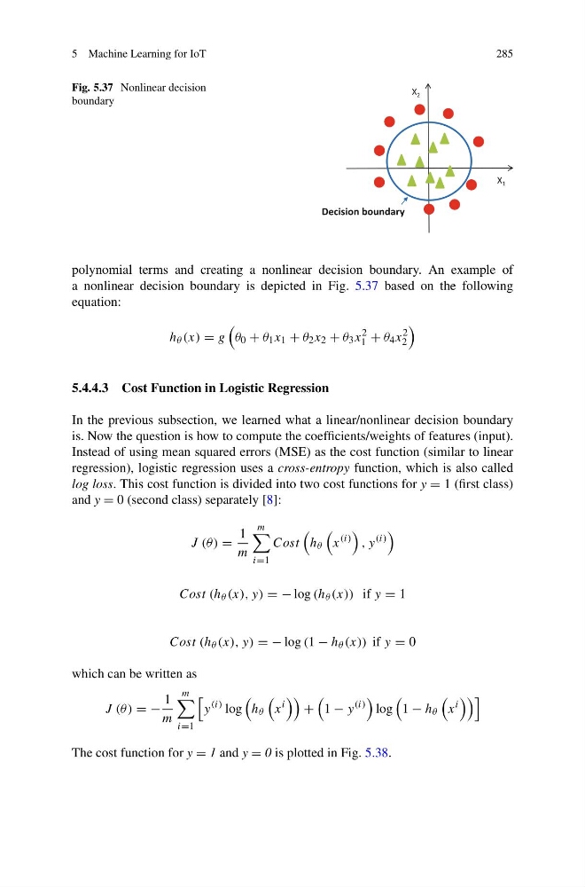
Fig. 5.37 Nonlinear decision
boundary
X 1
X 2
Decision boundary
polynomial terms and creating a nonlinear decision boundary. An example of
a nonlinear decision boundary is depicted in Fig. 5.37 based on the following
equation:
h θ (x) = g
θ 0 + θ 1 x 1 + θ 2 x 2 + θ 3 x
2
1 + θ 4 x
2
2
5.4.4.3 Cost Function in Logistic Regression
In the previous subsection, we learned what a linear/nonlinear decision boundary
is. Now the question is how to compute the coefficients/weights of features (input).
Instead of using mean squared errors (MSE) as the cost function (similar to linear
regression), logistic regression uses a cross-entropy function, which is also called
log loss. This cost function is divided into two cost functions for y = 1 (first class)
and y = 0 (second class) separately [8]:
J (θ ) =
1
m
m
i=1
Cost
h θ
x
(i)
, y
(i)
Cost (h θ (x), y) = − log (h θ (x)) if y = 1
Cost (h θ (x), y) = − log (1 − h θ (x)) if y = 0
which can be written as
J (θ ) = −
1
m
m
i=1
y
(i) log
h θ
x
i
+
1 − y
(i)
log
1 − h θ
x
i
The cost function for y = 1 and y = 0 is plotted in Fig. 5.38.
285
Fig. 5.37 Nonlinear decision
boundary
X 1
X 2
Decision boundary
polynomial terms and creating a nonlinear decision boundary. An example of
a nonlinear decision boundary is depicted in Fig. 5.37 based on the following
equation:
h θ (x) = g
θ 0 + θ 1 x 1 + θ 2 x 2 + θ 3 x
2
1 + θ 4 x
2
2
5.4.4.3 Cost Function in Logistic Regression
In the previous subsection, we learned what a linear/nonlinear decision boundary
is. Now the question is how to compute the coefficients/weights of features (input).
Instead of using mean squared errors (MSE) as the cost function (similar to linear
regression), logistic regression uses a cross-entropy function, which is also called
log loss. This cost function is divided into two cost functions for y = 1 (first class)
and y = 0 (second class) separately [8]:
J (θ ) =
1
m
m
i=1
Cost
h θ
x
(i)
, y
(i)
Cost (h θ (x), y) = − log (h θ (x)) if y = 1
Cost (h θ (x), y) = − log (1 − h θ (x)) if y = 0
which can be written as
J (θ ) = −
1
m
m
i=1
y
(i) log
h θ
x
i
+
1 − y
(i)
log
1 − h θ
x
i
The cost function for y = 1 and y = 0 is plotted in Fig. 5.38.