

284
F. Firouzi et al.
5.4.4.2 Decision Boundary (Decision Surface)
In order to map the returned score of the logistic function (which is a probability
in the range of [0,1]) to a binary class, a threshold is defined, above which the
classification output would be the class 1; otherwise the class would be 0. For
example, when the threshold is 0.5, classes can be identified by the following rule
(see Fig. 5.35):
Class = 1 : h θ (x) ≥ 0.5,
Class = 0 : h θ (x) < 0.5
Now, let us explain the meaning of the decision boundary by an example. Recall
that h θ (x) = g(θ T x) in which g() is a sigmoid (logistic) function and x represents the
input (features). When the threshold value is equal to 0.5, according to Fig. 5.35, it
implies that
Class = 1 : θ
T x ≥ 0,
Class = 0 : θ
T x < 0
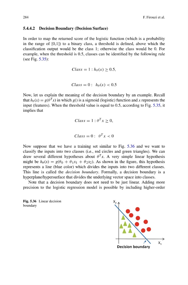
Now suppose that we have a training set similar to Fig. 5.36 and we want to
classify the inputs into two classes (i.e., red circles and green triangles). We can
draw several different hypotheses about θ T x. A very simple linear hypothesis
might be h θ (x) = g(θ 0 + θ 1 x 1 + θ 2 x 2 ). As shown in the figure, this hypothesis
represents a line (blue color) which divides the inputs into two different classes.
This line is called the decision boundary. Formally, a decision boundary is a
hyperplane/hypersurface that divides the underlying vector space into classes.
Note that a decision boundary does not need to be just linear. Adding more
precision to the logistic regression model is possible by including higher-order
Fig. 5.36 Linear decision
boundary
X 1
X 2
Decision boundary
F. Firouzi et al.
5.4.4.2 Decision Boundary (Decision Surface)
In order to map the returned score of the logistic function (which is a probability
in the range of [0,1]) to a binary class, a threshold is defined, above which the
classification output would be the class 1; otherwise the class would be 0. For
example, when the threshold is 0.5, classes can be identified by the following rule
(see Fig. 5.35):
Class = 1 : h θ (x) ≥ 0.5,
Class = 0 : h θ (x) < 0.5
Now, let us explain the meaning of the decision boundary by an example. Recall
that h θ (x) = g(θ T x) in which g() is a sigmoid (logistic) function and x represents the
input (features). When the threshold value is equal to 0.5, according to Fig. 5.35, it
implies that
Class = 1 : θ
T x ≥ 0,
Class = 0 : θ
T x < 0
Now suppose that we have a training set similar to Fig. 5.36 and we want to
classify the inputs into two classes (i.e., red circles and green triangles). We can
draw several different hypotheses about θ T x. A very simple linear hypothesis
might be h θ (x) = g(θ 0 + θ 1 x 1 + θ 2 x 2 ). As shown in the figure, this hypothesis
represents a line (blue color) which divides the inputs into two different classes.
This line is called the decision boundary. Formally, a decision boundary is a
hyperplane/hypersurface that divides the underlying vector space into classes.
Note that a decision boundary does not need to be just linear. Adding more
precision to the logistic regression model is possible by including higher-order
Fig. 5.36 Linear decision
boundary
X 1
X 2
Decision boundary