

3.2 One-Dimensional Analysis Model
27
III
Sink
I
I
I
IV
1
c
Q disp
4
c
Q cont
2
c
3
c
2
1
Q
Q 4
3
Q
Q
III
Sink
I
I
I
IV
1
c
Q disp
4
c
Q cont
2
c
3
c
4
Q 1
2
Q
3
Q
Q
(a) Without droplets
(b) With droplets
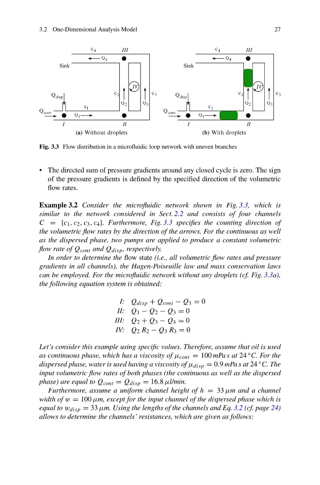
Fig. 3.3 Flow distribution in a microfluidic loop network with uneven branches
• The directed sum of pressure gradients around any closed cycle is zero. The sign
of the pressure gradients is defined by the specified direction of the volumetric
flow rates.
Example 3.2 Consider the microfluidic network shown in Fig. 3.3, which is
similar to the network considered in Sect. 2.2 and consists of four channels
C = {c 1 , c 2 , c 3 , c 4 }. Furthermore, Fig. 3.3 specifies the counting direction of
the volumetric flow rates by the direction of the arrows. For the continuous as well
as the dispersed phase, two pumps are applied to produce a constant volumetric
flow rate of Q cont and Q disp , respectively.
In order to determine the flow state (i.e., all volumetric flow rates and pressure
gradients in all channels), the Hagen-Poiseuille law and mass conservation laws
can be employed. For the microfluidic network without any droplets (cf. Fig. 3.3a),
the following equation system is obtained:
I: Q disp + Q cont − Q 1 = 0
II: Q 1 − Q 2 − Q 3 = 0
III: Q 2 + Q 3 − Q 4 = 0
IV: Q 2 R 2 − Q 3 R 3 = 0
Let’s consider this example using specific values. Therefore, assume that oil is used
as continuous phase, which has a viscosity of μ cont = 100 mPa s at 24 ◦ C. For the
dispersed phase, water is used having a viscosity of μ disp = 0.9 mPa s at 24 ◦ C. The
input volumetric flow rates of both phases (the continuous as well as the dispersed
phase) are equal to Q cont = Q disp = 16.8 μl/min.
Furthermore, assume a uniform channel height of h = 33 μm and a channel
width of w = 100 μm, except for the input channel of the dispersed phase which is
equal to w disp = 33 μm. Using the lengths of the channels and Eq. 3.2 (cf. page 24)
allows to determine the channels’ resistances, which are given as follows:
27
III
Sink
I
I
I
IV
1
c
Q disp
4
c
Q cont
2
c
3
c
2
1
Q
Q 4
3
Q
Q
III
Sink
I
I
I
IV
1
c
Q disp
4
c
Q cont
2
c
3
c
4
Q 1
2
Q
3
Q
Q
(a) Without droplets
(b) With droplets
Fig. 3.3 Flow distribution in a microfluidic loop network with uneven branches
• The directed sum of pressure gradients around any closed cycle is zero. The sign
of the pressure gradients is defined by the specified direction of the volumetric
flow rates.
Example 3.2 Consider the microfluidic network shown in Fig. 3.3, which is
similar to the network considered in Sect. 2.2 and consists of four channels
C = {c 1 , c 2 , c 3 , c 4 }. Furthermore, Fig. 3.3 specifies the counting direction of
the volumetric flow rates by the direction of the arrows. For the continuous as well
as the dispersed phase, two pumps are applied to produce a constant volumetric
flow rate of Q cont and Q disp , respectively.
In order to determine the flow state (i.e., all volumetric flow rates and pressure
gradients in all channels), the Hagen-Poiseuille law and mass conservation laws
can be employed. For the microfluidic network without any droplets (cf. Fig. 3.3a),
the following equation system is obtained:
I: Q disp + Q cont − Q 1 = 0
II: Q 1 − Q 2 − Q 3 = 0
III: Q 2 + Q 3 − Q 4 = 0
IV: Q 2 R 2 − Q 3 R 3 = 0
Let’s consider this example using specific values. Therefore, assume that oil is used
as continuous phase, which has a viscosity of μ cont = 100 mPa s at 24 ◦ C. For the
dispersed phase, water is used having a viscosity of μ disp = 0.9 mPa s at 24 ◦ C. The
input volumetric flow rates of both phases (the continuous as well as the dispersed
phase) are equal to Q cont = Q disp = 16.8 μl/min.
Furthermore, assume a uniform channel height of h = 33 μm and a channel
width of w = 100 μm, except for the input channel of the dispersed phase which is
equal to w disp = 33 μm. Using the lengths of the channels and Eq. 3.2 (cf. page 24)
allows to determine the channels’ resistances, which are given as follows: