

266
25 Elastic Displacements and Waves
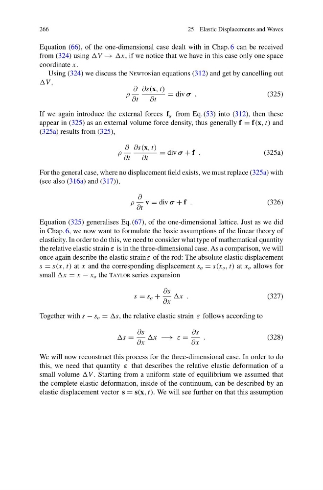
Equation (66), of the one-dimensional case dealt with in Chap. 6 can be received
from (324) using V → x, if we notice that we have in this case only one space
coordinate x.
Using (324) we discuss the Newtonian equations (312) and get by cancelling out
V ,
ρ
∂
∂t
∂s(x, t)
∂t
= div σ .
(325)
If we again introduce the external forces f a from Eq. (53) into (312), then these
appear in (325) as an external volume force density, thus generally f = f(x, t) and
(325a) results from (325),
ρ
∂
∂t
∂s(x, t)
∂t
= div σ + f .
(325a)
For the general case, where no displacement field exists, we must replace (325a) with
(see also (316a) and (317)),
ρ
∂
∂t
v = div σ + f .
(326)
Equation (325) generalises Eq. (67), of the one-dimensional lattice. Just as we did
in Chap. 6, we now want to formulate the basic assumptions of the linear theory of
elasticity. In order to do this, we need to consider what type of mathematical quantity
the relative elastic strain ε is in the three-dimensional case. As a comparison, we will
once again describe the elastic strain ε of the rod: The absolute elastic displacement
s = s(x, t) at x and the corresponding displacement s o = s(x o , t) at x o allows for
small x = x − x o the Taylor series expansion
s = s o +
∂s
∂x
x .
(327)
Together with s − s o = s, the relative elastic strain ε follows according to
s =
∂s
∂x
x −→ ε =
∂s
∂x
.
(328)
We will now reconstruct this process for the three-dimensional case. In order to do
this, we need that quantity ε that describes the relative elastic deformation of a
small volume V . Starting from a uniform state of equilibrium we assumed that
the complete elastic deformation, inside of the continuum, can be described by an
elastic displacement vector s = s(x, t). We will see further on that this assumption
25 Elastic Displacements and Waves
Equation (66), of the one-dimensional case dealt with in Chap. 6 can be received
from (324) using V → x, if we notice that we have in this case only one space
coordinate x.
Using (324) we discuss the Newtonian equations (312) and get by cancelling out
V ,
ρ
∂
∂t
∂s(x, t)
∂t
= div σ .
(325)
If we again introduce the external forces f a from Eq. (53) into (312), then these
appear in (325) as an external volume force density, thus generally f = f(x, t) and
(325a) results from (325),
ρ
∂
∂t
∂s(x, t)
∂t
= div σ + f .
(325a)
For the general case, where no displacement field exists, we must replace (325a) with
(see also (316a) and (317)),
ρ
∂
∂t
v = div σ + f .
(326)
Equation (325) generalises Eq. (67), of the one-dimensional lattice. Just as we did
in Chap. 6, we now want to formulate the basic assumptions of the linear theory of
elasticity. In order to do this, we need to consider what type of mathematical quantity
the relative elastic strain ε is in the three-dimensional case. As a comparison, we will
once again describe the elastic strain ε of the rod: The absolute elastic displacement
s = s(x, t) at x and the corresponding displacement s o = s(x o , t) at x o allows for
small x = x − x o the Taylor series expansion
s = s o +
∂s
∂x
x .
(327)
Together with s − s o = s, the relative elastic strain ε follows according to
s =
∂s
∂x
x −→ ε =
∂s
∂x
.
(328)
We will now reconstruct this process for the three-dimensional case. In order to do
this, we need that quantity ε that describes the relative elastic deformation of a
small volume V . Starting from a uniform state of equilibrium we assumed that
the complete elastic deformation, inside of the continuum, can be described by an
elastic displacement vector s = s(x, t). We will see further on that this assumption