

30
28
26
24
22
20
18
16
14
12
10
8
6
4
2
0
Differential Capacitance, μF/cm
2
–0.4
–0.3
–0.2
–0.1
0
0.1
0.2
0.3
0.4
Potential Across the Diffuse Layer, V
Capacitance of the Helmholtz layer
0.01 M, Capacitance of the entire double-layer
0.00001 M, Capacitance of the entire
1.0 M, Capacitance of the entire double-layer
double-layer
5.0 M, Capacitance of the entire double-layer
49
Fundamentals of Electrochemical Double-Layer Supercapacitors
ε ε
C
r o
H =
,
d
in which the thickness of the Helmholtz layer (d) is about the diameter of a
water molecule, ~1.9 ×10 –10 m. The high electric field within the Helmholtz
layer (>10 9 V.m –1 ) can make all polarities of the water molecules in order,
leading to a smaller relative dielectric constant (~ 6) than that of randomly
distributed water, which is about 40 in the presence of an electrolyte. The
calculated C H value is about 28 μF.cm –2 . If C H = 28 μF.cm –2 , ε = 40 (aqueous
electrolyte solution), z = 1, and T = 25°C, then C dl can be calculated according to Equation (2.19). The obtained differential capacitance data at different
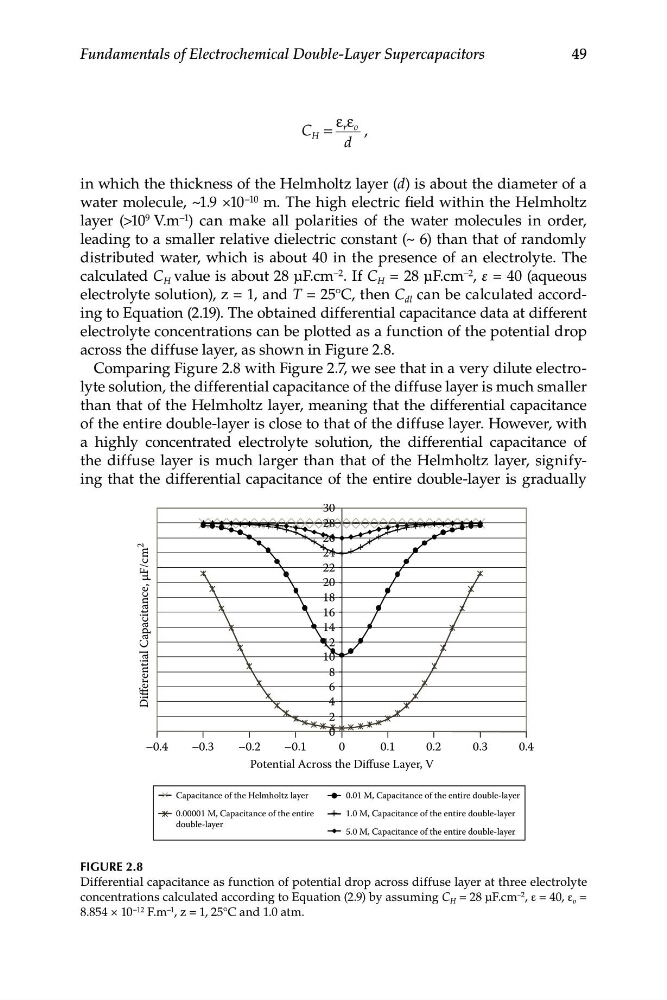
electrolyte concentrations can be plotted as a function of the potential drop
across the diffuse layer, as shown in Figure 2.8.
Comparing Figure 2.8 with Figure 2.7, we see that in a very dilute electrolyte solution, the differential capacitance of the diffuse layer is much smaller
than that of the Helmholtz layer, meaning that the differential capacitance
of the entire double-layer is close to that of the diffuse layer. However, with
a highly concentrated electrolyte solution, the differential capacitance of
the diffuse layer is much larger than that of the Helmholtz layer, signifying that the differential capacitance of the entire double-layer is gradually
FIGURE 2.8
Differential capacitance as function of potential drop across diffuse layer at three electrolyte
concentrations calculated according to Equation (2.9) by assuming C H = 28 μF.cm –2 , ε = 40, ε o =
8.854 × 10 −12 F.m –1 , z = 1, 25°C and 1.0 atm.
28
26
24
22
20
18
16
14
12
10
8
6
4
2
0
Differential Capacitance, μF/cm
2
–0.4
–0.3
–0.2
–0.1
0
0.1
0.2
0.3
0.4
Potential Across the Diffuse Layer, V
Capacitance of the Helmholtz layer
0.01 M, Capacitance of the entire double-layer
0.00001 M, Capacitance of the entire
1.0 M, Capacitance of the entire double-layer
double-layer
5.0 M, Capacitance of the entire double-layer
49
Fundamentals of Electrochemical Double-Layer Supercapacitors
ε ε
C
r o
H =
,
d
in which the thickness of the Helmholtz layer (d) is about the diameter of a
water molecule, ~1.9 ×10 –10 m. The high electric field within the Helmholtz
layer (>10 9 V.m –1 ) can make all polarities of the water molecules in order,
leading to a smaller relative dielectric constant (~ 6) than that of randomly
distributed water, which is about 40 in the presence of an electrolyte. The
calculated C H value is about 28 μF.cm –2 . If C H = 28 μF.cm –2 , ε = 40 (aqueous
electrolyte solution), z = 1, and T = 25°C, then C dl can be calculated according to Equation (2.19). The obtained differential capacitance data at different
electrolyte concentrations can be plotted as a function of the potential drop
across the diffuse layer, as shown in Figure 2.8.
Comparing Figure 2.8 with Figure 2.7, we see that in a very dilute electrolyte solution, the differential capacitance of the diffuse layer is much smaller
than that of the Helmholtz layer, meaning that the differential capacitance
of the entire double-layer is close to that of the diffuse layer. However, with
a highly concentrated electrolyte solution, the differential capacitance of
the diffuse layer is much larger than that of the Helmholtz layer, signifying that the differential capacitance of the entire double-layer is gradually
FIGURE 2.8
Differential capacitance as function of potential drop across diffuse layer at three electrolyte
concentrations calculated according to Equation (2.9) by assuming C H = 28 μF.cm –2 , ε = 40, ε o =
8.854 × 10 −12 F.m –1 , z = 1, 25°C and 1.0 atm.