

301
Characterization and Diagnosis Techniques
C dl
+
–
R esr
C F
R ct
R P
(a)
+
–
R 1
R 2
R n–1
C n–1
C 2
C 1
R n
C n
(b)
+
R 1
R 2
R n–1
R n
–
Q n–1
Q 2
Q 1
Q n
(c)
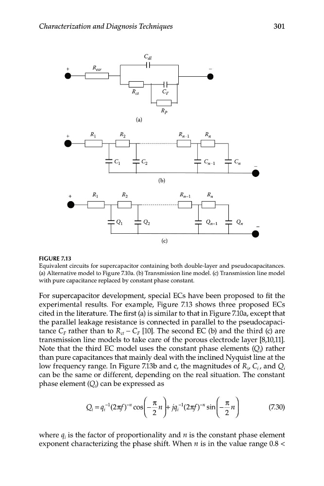
FIGURE 7.13
Equivalent circuits for supercapacitor containing both double-layer and pseudocapacitances.
(a) Alternative model to Figure 7.10a. (b) Transmission line model. (c) Transmission line model
with pure capacitance replaced by constant phase constant.
For supercapacitor development, special ECs have been proposed to fit the
experimental results. For example, Figure 7.13 shows three proposed ECs
cited in the literature. The first (a) is similar to that in Figure 7.10a, except that
the parallel leakage resistance is connected in parallel to the pseudocapacitance C F rather than to R ct – C F [10]. The second EC (b) and the third (c) are
transmission line models to take care of the porous electrode layer [8,10,11].
Note that the third EC model uses the constant phase elements (Q i ) rather
than pure capacitances that mainly deal with the inclined Nyquist line at the
low frequency range. In Figure 7.13b and c, the magnitudes of R i , C i , and Q i
can be the same or different, depending on the real situation. The constant
phase element (Q i ) can be expressed as
Q q
=
−1
⎞
⎛ π
i
πf
−n
⎛ π
⎞
i (2 ) cos ⎜ − n ⎟ + jq
−1 (2 f )
− n
i
π
sin ⎜ − − n ⎟
(7.30)
⎝ 2 ⎠
⎝ 2 ⎠
where q i is the factor of proportionality and n is the constant phase element
exponent characterizing the phase shift. When n is in the value range 0.8 <
Characterization and Diagnosis Techniques
C dl
+
–
R esr
C F
R ct
R P
(a)
+
–
R 1
R 2
R n–1
C n–1
C 2
C 1
R n
C n
(b)
+
R 1
R 2
R n–1
R n
–
Q n–1
Q 2
Q 1
Q n
(c)
FIGURE 7.13
Equivalent circuits for supercapacitor containing both double-layer and pseudocapacitances.
(a) Alternative model to Figure 7.10a. (b) Transmission line model. (c) Transmission line model
with pure capacitance replaced by constant phase constant.
For supercapacitor development, special ECs have been proposed to fit the
experimental results. For example, Figure 7.13 shows three proposed ECs
cited in the literature. The first (a) is similar to that in Figure 7.10a, except that
the parallel leakage resistance is connected in parallel to the pseudocapacitance C F rather than to R ct – C F [10]. The second EC (b) and the third (c) are
transmission line models to take care of the porous electrode layer [8,10,11].
Note that the third EC model uses the constant phase elements (Q i ) rather
than pure capacitances that mainly deal with the inclined Nyquist line at the
low frequency range. In Figure 7.13b and c, the magnitudes of R i , C i , and Q i
can be the same or different, depending on the real situation. The constant
phase element (Q i ) can be expressed as
Q q
=
−1
⎞
⎛ π
i
πf
−n
⎛ π
⎞
i (2 ) cos ⎜ − n ⎟ + jq
−1 (2 f )
− n
i
π
sin ⎜ − − n ⎟
(7.30)
⎝ 2 ⎠
⎝ 2 ⎠
where q i is the factor of proportionality and n is the constant phase element
exponent characterizing the phase shift. When n is in the value range 0.8 <