

298
Electrochemical Supercapacitors for Energy Storage and Delivery
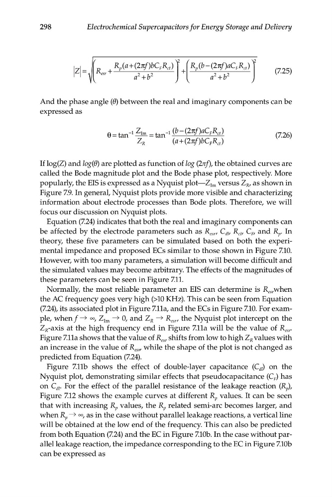
⎛
R a
( + (2 πf )b C R ) ⎞
2 ⎛
p
F ct
R b
( − − (2 π
2
p
f a
) C
⎞
Z = ⎜R +
⎟ + ⎜
F c
R t )
⎜ esr
2
⎟
⎟
(7.25)
⎝
a + b
2
⎜
⎠ ⎝
a
2
⎟
+ b
2
⎠
And the phase angle (θ) between the real and imaginary components can be
expressed as
−1 Z Im
−1 (b − (2πf ) aC F c
R )
θ = tan
= tan
t
(7.26)
Z R
(a + (2πf )b C F F c
R t )
If log(Z) and log(θ) are plotted as function of log (2πf), the obtained curves are
called the Bode magnitude plot and the Bode phase plot, respectively. More
popularly, the EIS is expressed as a Nyquist plot—Z Im versus Z R , as shown in
Figure 7.9. In general, Nyquist plots provide more visible and characterizing
information about electrode processes than Bode plots. Therefore, we will
focus our discussion on Nyquist plots.
Equation (7.24) indicates that both the real and imaginary components can
be affected by the electrode parameters such as R esr , C dl , R ct , C F , and R p . In
theory, these five parameters can be simulated based on both the experimental impedance and proposed ECs similar to those shown in Figure 7.10.
However, with too many parameters, a simulation will become difficult and
the simulated values may become arbitrary. The effects of the magnitudes of
these parameters can be seen in Figure 7.11.
Normally, the most reliable parameter an EIS can determine is R esr when
the AC frequency goes very high (>10 KHz). This can be seen from Equation
(7.24), its associated plot in Figure 7.11a, and the ECs in Figure 7.10. For example, when f → ∞, Z Im → 0, and Z R → R esr , the Nyquist plot intercept on the
Z R -axis at the high frequency end in Figure 7.11a will be the value of R esr .
Figure 7.11a shows that the value of R esr shifts from low to high Z R values with
an increase in the value of R esr , while the shape of the plot is not changed as
predicted from Equation (7.24).
Figure 7.11b shows the effect of double-layer capacitance (C dl ) on the
Nyquist plot, demonstrating similar effects that pseudocapacitance (C F ) has
on C dl . For the effect of the parallel resistance of the leakage reaction (R p ),
Figure 7.12 shows the example curves at different R p values. It can be seen
that with increasing R p values, the R p related semi-arc becomes larger, and
when R p → ∞, as in the case without parallel leakage reactions, a vertical line
will be obtained at the low end of the frequency. This can also be predicted
from both Equation (7.24) and the EC in Figure 7.10b. In the case without parallel leakage reaction, the impedance corresponding to the EC in Figure 7.10b
can be expressed as
Electrochemical Supercapacitors for Energy Storage and Delivery
⎛
R a
( + (2 πf )b C R ) ⎞
2 ⎛
p
F ct
R b
( − − (2 π
2
p
f a
) C
⎞
Z = ⎜R +
⎟ + ⎜
F c
R t )
⎜ esr
2
⎟
⎟
(7.25)
⎝
a + b
2
⎜
⎠ ⎝
a
2
⎟
+ b
2
⎠
And the phase angle (θ) between the real and imaginary components can be
expressed as
−1 Z Im
−1 (b − (2πf ) aC F c
R )
θ = tan
= tan
t
(7.26)
Z R
(a + (2πf )b C F F c
R t )
If log(Z) and log(θ) are plotted as function of log (2πf), the obtained curves are
called the Bode magnitude plot and the Bode phase plot, respectively. More
popularly, the EIS is expressed as a Nyquist plot—Z Im versus Z R , as shown in
Figure 7.9. In general, Nyquist plots provide more visible and characterizing
information about electrode processes than Bode plots. Therefore, we will
focus our discussion on Nyquist plots.
Equation (7.24) indicates that both the real and imaginary components can
be affected by the electrode parameters such as R esr , C dl , R ct , C F , and R p . In
theory, these five parameters can be simulated based on both the experimental impedance and proposed ECs similar to those shown in Figure 7.10.
However, with too many parameters, a simulation will become difficult and
the simulated values may become arbitrary. The effects of the magnitudes of
these parameters can be seen in Figure 7.11.
Normally, the most reliable parameter an EIS can determine is R esr when
the AC frequency goes very high (>10 KHz). This can be seen from Equation
(7.24), its associated plot in Figure 7.11a, and the ECs in Figure 7.10. For example, when f → ∞, Z Im → 0, and Z R → R esr , the Nyquist plot intercept on the
Z R -axis at the high frequency end in Figure 7.11a will be the value of R esr .
Figure 7.11a shows that the value of R esr shifts from low to high Z R values with
an increase in the value of R esr , while the shape of the plot is not changed as
predicted from Equation (7.24).
Figure 7.11b shows the effect of double-layer capacitance (C dl ) on the
Nyquist plot, demonstrating similar effects that pseudocapacitance (C F ) has
on C dl . For the effect of the parallel resistance of the leakage reaction (R p ),
Figure 7.12 shows the example curves at different R p values. It can be seen
that with increasing R p values, the R p related semi-arc becomes larger, and
when R p → ∞, as in the case without parallel leakage reactions, a vertical line
will be obtained at the low end of the frequency. This can also be predicted
from both Equation (7.24) and the EC in Figure 7.10b. In the case without parallel leakage reaction, the impedance corresponding to the EC in Figure 7.10b
can be expressed as