

Metal electrode (M)
Electrolyte solution
(S)
+ Positive charge
+
+
–
– Negative charge
+
–
Solvent molecule
–
+
+
–
–
+
–
+
–
+
–
–
+
–
+
d
(a)
Δφ m/s (=Δψ m/s )
Δφ m/s – Δφ H/s (=Δψ m/s –ψ 1 )
d
Δφ H/s (=Δψ 1 )
0
x
(b)
Positive charge
Negative charge
Solvent molecule
Electrolyte solution
Electrode
+
+
–
–
–
–
–
–
–
–
–
–
–
–
–
–
–
–
–
–
–
–
–
–
–
–
–
–
–
–
–
–
–
–
+
+
+
+
+
+
+
+
+
+
+
+
+
+
+
+
+
+
+
+
+
+
+
+
+
+
+
+
+
L diff
d IHP
d OHP
L diff
OHP
IHP
(c)
(b)
(a)
d
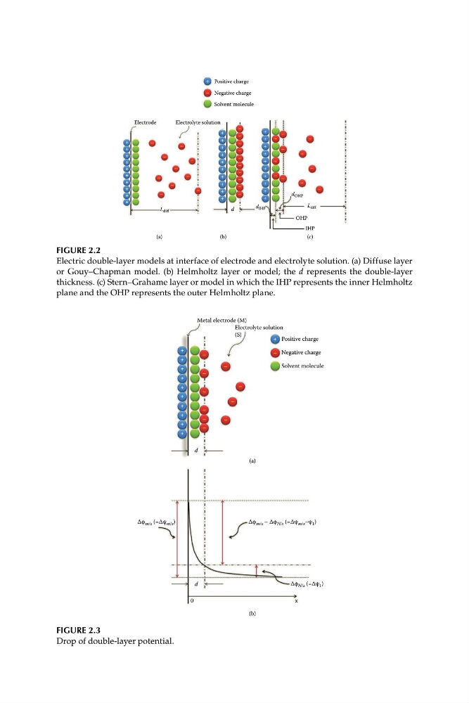
FIGURE 2.2
Electric double-layer models at interface of electrode and electrolyte solution. (a) Diffuse layer
or Gouy–Chapman model. (b) Helmholtz layer or model; the d represents the double-layer
thickness. (c) Stern–Grahame layer or model in which the IHP represents the inner Helmholtz
plane and the OHP represents the outer Helmholtz plane.
FIGURE 2.3
Drop of double-layer potential.
Electrolyte solution
(S)
+ Positive charge
+
+
–
– Negative charge
+
–
Solvent molecule
–
+
+
–
–
+
–
+
–
+
–
–
+
–
+
d
(a)
Δφ m/s (=Δψ m/s )
Δφ m/s – Δφ H/s (=Δψ m/s –ψ 1 )
d
Δφ H/s (=Δψ 1 )
0
x
(b)
Positive charge
Negative charge
Solvent molecule
Electrolyte solution
Electrode
+
+
–
–
–
–
–
–
–
–
–
–
–
–
–
–
–
–
–
–
–
–
–
–
–
–
–
–
–
–
–
–
–
–
+
+
+
+
+
+
+
+
+
+
+
+
+
+
+
+
+
+
+
+
+
+
+
+
+
+
+
+
+
L diff
d IHP
d OHP
L diff
OHP
IHP
(c)
(b)
(a)
d
FIGURE 2.2
Electric double-layer models at interface of electrode and electrolyte solution. (a) Diffuse layer
or Gouy–Chapman model. (b) Helmholtz layer or model; the d represents the double-layer
thickness. (c) Stern–Grahame layer or model in which the IHP represents the inner Helmholtz
plane and the OHP represents the outer Helmholtz plane.
FIGURE 2.3
Drop of double-layer potential.