

105
Fundamentals of Electrochemical Pseudocapacitors
⎛
⎞
⎜
⎟
o
⎜
1
⎟
C O X = C O X ⎜
⎟
(3.8)
⎛
⎞
⎜
nF
⎟
⎜
xp
(E
o
C
1 e
+
⎜
O /R − E) +
⎝
d
g
O X ⎟
⎜
X
o ⎟ ⎟
⎝
RT
C O X ⎠ ⎠ ⎠
Equation (3.6) can then be alternatively expressed as
n F
2 2
C E
( ) =
dC
o
pc
RT
O X
⎛ nF o
C ⎞
ex
(
O
p ⎜
E
− +
E) g
⎜
X ⎟
RT
O X /R d
⎟
(3.9)
⎝
C
o
O X X ⎠
⎡
⎛
C ⎞⎤
2
⎛
⎞
nF (E
o
nF
C
⎢ 1 e
+ xp ⎜
O /R − E) + g
O X ⎟⎥ + g exp ⎜
(E
o
O /R − E) + g
O
⎜
X ⎟
⎜
X
d
o ⎟
⎜
X
d
o o ⎟
⎢ ⎣
⎝ RT
C O X ⎠ ⎥
⎦
⎝ RT
C O X ⎠
Equation (3.9) will be converted into Equation (3.6) when g = 0 and the situation corresponds to a completely reversible redox reaction. If g > 0, the redox
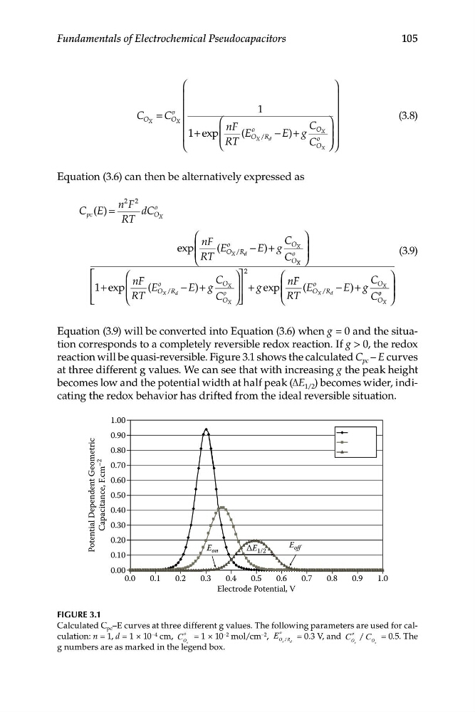
reaction will be quasi-reversible. Figure 3.1 shows the calculated C pc – E curves
at three different g values. We can see that with increasing g the peak height
becomes low and the potential width at half peak (ΔE 1/2 ) becomes wider, indicating the redox behavior has drifted from the ideal reversible situation.
1.00
0.90
g = 0
ometric
g = 5
0.80
g = 15
–2
e
0.70
t G
.
e, F cm
ial Dependen
0.60
pacitanc
0.50
0.40
a
C
0.30
tent
o
0.20
P
E
ΔE
E off
0.10
on
1/2
0.00
0.0 0.1
0.2
0.3
0.4
0.5
0.6
0.7
0.8
0.9
1.0
Electrode Potential, V
FIGURE 3.1
Calculated C pc –E curves at three different g values. The following parameters are used for calculation: n = 1, d = 1 × 10 –4 cm, C
o = 1 × 10 –2 mol/cm –2 , E
o
O
O R
/
= 0 .3 V, and C
o
O
/ C O = 0.5. The
g numbers are as marked in the le
x
d
x
gend box.
x
x
Fundamentals of Electrochemical Pseudocapacitors
⎛
⎞
⎜
⎟
o
⎜
1
⎟
C O X = C O X ⎜
⎟
(3.8)
⎛
⎞
⎜
nF
⎟
⎜
xp
(E
o
C
1 e
+
⎜
O /R − E) +
⎝
d
g
O X ⎟
⎜
X
o ⎟ ⎟
⎝
RT
C O X ⎠ ⎠ ⎠
Equation (3.6) can then be alternatively expressed as
n F
2 2
C E
( ) =
dC
o
pc
RT
O X
⎛ nF o
C ⎞
ex
(
O
p ⎜
E
− +
E) g
⎜
X ⎟
RT
O X /R d
⎟
(3.9)
⎝
C
o
O X X ⎠
⎡
⎛
C ⎞⎤
2
⎛
⎞
nF (E
o
nF
C
⎢ 1 e
+ xp ⎜
O /R − E) + g
O X ⎟⎥ + g exp ⎜
(E
o
O /R − E) + g
O
⎜
X ⎟
⎜
X
d
o ⎟
⎜
X
d
o o ⎟
⎢ ⎣
⎝ RT
C O X ⎠ ⎥
⎦
⎝ RT
C O X ⎠
Equation (3.9) will be converted into Equation (3.6) when g = 0 and the situation corresponds to a completely reversible redox reaction. If g > 0, the redox
reaction will be quasi-reversible. Figure 3.1 shows the calculated C pc – E curves
at three different g values. We can see that with increasing g the peak height
becomes low and the potential width at half peak (ΔE 1/2 ) becomes wider, indicating the redox behavior has drifted from the ideal reversible situation.
1.00
0.90
g = 0
ometric
g = 5
0.80
g = 15
–2
e
0.70
t G
.
e, F cm
ial Dependen
0.60
pacitanc
0.50
0.40
a
C
0.30
tent
o
0.20
P
E
ΔE
E off
0.10
on
1/2
0.00
0.0 0.1
0.2
0.3
0.4
0.5
0.6
0.7
0.8
0.9
1.0
Electrode Potential, V
FIGURE 3.1
Calculated C pc –E curves at three different g values. The following parameters are used for calculation: n = 1, d = 1 × 10 –4 cm, C
o = 1 × 10 –2 mol/cm –2 , E
o
O
O R
/
= 0 .3 V, and C
o
O
/ C O = 0.5. The
g numbers are as marked in the le
x
d
x
gend box.
x
x