

Exercises
65
2 DG
2 J
2
<
&(SRURXV3W
:(
VDPSOH/6&R
3WFROOHFWRU
HQFDSVXODWLRQJODVV
SRWHQWLRVWDW
<6=PLFURSRLQW
2
<
H
<
2
<
D
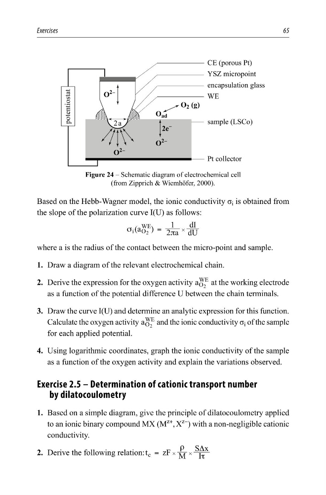
Figure 24 – Schematic diagram of electrochemical cell
(from Zipprich & Wiemhöfer, 2000).
Based on the Hebb-Wagner model, the ionic conductivity σ i is obtained from
the slope of the polarization curve I(U) as follows:
(a )
2 a
1
dU
dI
i O
WE
2
σ
π
=
#
where a is the radius of the contact between the micro-point and sample.
1. Draw a diagram of the relevant electrochemical chain.
2. Derive the expression for the oxygen activity a O
WE
2
at the working electrode
as a function of the potential difference U between the chain terminals.
3. Draw the curve I(U) and determine an analytic expression for this function.
Calculate the oxygen activity a O
WE
2
and the ionic conductivity σ i of the sample
for each applied potential.
4. Using logarithmic coordinates, graph the ionic conductivity of the sample
as a function of the oxygen activity and explain the variations observed.
Exercise 2.5 – Determination of cationic transport number
by dilatocoulometry
1. Based on a simple diagram, give the principle of dilatocoulometry applied
to an ionic binary compound MX (M
z+
, X
z−
) with a non-negligible cationic
conductivity.
2. Derive the following relation: t
zF M
I
S x
c
ρ
τ
Δ
=
#
#
65
2 DG
2 J
2
<
&(SRURXV3W
:(
VDPSOH/6&R
3WFROOHFWRU
HQFDSVXODWLRQJODVV
SRWHQWLRVWDW
<6=PLFURSRLQW
2
<
H
<
2
<
D
Figure 24 – Schematic diagram of electrochemical cell
(from Zipprich & Wiemhöfer, 2000).
Based on the Hebb-Wagner model, the ionic conductivity σ i is obtained from
the slope of the polarization curve I(U) as follows:
(a )
2 a
1
dU
dI
i O
WE
2
σ
π
=
#
where a is the radius of the contact between the micro-point and sample.
1. Draw a diagram of the relevant electrochemical chain.
2. Derive the expression for the oxygen activity a O
WE
2
at the working electrode
as a function of the potential difference U between the chain terminals.
3. Draw the curve I(U) and determine an analytic expression for this function.
Calculate the oxygen activity a O
WE
2
and the ionic conductivity σ i of the sample
for each applied potential.
4. Using logarithmic coordinates, graph the ionic conductivity of the sample
as a function of the oxygen activity and explain the variations observed.
Exercise 2.5 – Determination of cationic transport number
by dilatocoulometry
1. Based on a simple diagram, give the principle of dilatocoulometry applied
to an ionic binary compound MX (M
z+
, X
z−
) with a non-negligible cationic
conductivity.
2. Derive the following relation: t
zF M
I
S x
c
ρ
τ
Δ
=
#
#