

Exercises
61
Table 13 – Electric characteristics determined at 300 °C.
Circuit
R [Ω]
C [F]
A [F s
p−1
]
p
R //C
6.07 # 10
4
2.93 # 10
−11
−
−
R //CPE
6.19 # 10
4
−
1.41 # 10
−10
0.879
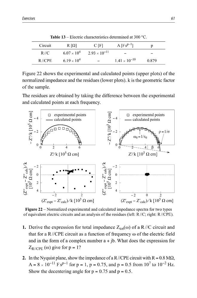
Figure 22 shows the experimental and calculated points (upper plots) of the
normalized impedance and the residues (lower plots). k is the geometric factor
of the sample.
The residues are obtained by taking the difference between the experimental
and calculated points at each frequency.
<
<
<
<
=ƍƍ
H[SW <=ƍƍ
FDOF » N
>
ȍFP@
=ƍƍ
H[SW <=ƍƍ
FDOF » N
>
ȍFP@
=ƍ H[SW <=ƍ FDOF » N>
ȍFP@
=ƍ H[SW <=ƍ FDOF » N>
ȍFP@
H[SHULPHQWDOSRLQWV
FDOFXODWHGSRLQWV
H[SHULPHQWDOSRLQWV
FDOFXODWHGSRLQWV
<
<
<
<
ȕ
ȡ ı
Ȧ IJ
=ƍ» N>
ȍ FP@
<
=ƍƍ» N>
ȍFP@
<
=ƍƍ» N>
ȍFP@
=ƍ» N>
ȍFP@
Figure 22 – Normalized experimental and calculated impedance spectra for two types
of equivalent electric circuits and an analysis of the residues (left: R //C; right: R //CPE).
1. Derive the expression for total impedance Z tot (ω) of a R //C circuit and
that for a R //CPE circuit as a function of frequency ω of the electric field
and in the form of a complex number a + jb. What does the expression for
Z R//CPE (ω) give for p = 1?
2. In the Nyquist plane, show the impedance of a R //CPE circuit with R = 0.8 MΩ,
A = 8 # 10
−11
F s
p−1
for p = 1, p = 0.75, and p = 0.5 from 10
7
to 10
−2
Hz.
Show the decentering angle for p = 0.75 and p = 0.5.
61
Table 13 – Electric characteristics determined at 300 °C.
Circuit
R [Ω]
C [F]
A [F s
p−1
]
p
R //C
6.07 # 10
4
2.93 # 10
−11
−
−
R //CPE
6.19 # 10
4
−
1.41 # 10
−10
0.879
Figure 22 shows the experimental and calculated points (upper plots) of the
normalized impedance and the residues (lower plots). k is the geometric factor
of the sample.
The residues are obtained by taking the difference between the experimental
and calculated points at each frequency.
<
<
<
<
=ƍƍ
H[SW <=ƍƍ
FDOF » N
>
ȍFP@
=ƍƍ
H[SW <=ƍƍ
FDOF » N
>
ȍFP@
=ƍ H[SW <=ƍ FDOF » N>
ȍFP@
=ƍ H[SW <=ƍ FDOF » N>
ȍFP@
H[SHULPHQWDOSRLQWV
FDOFXODWHGSRLQWV
H[SHULPHQWDOSRLQWV
FDOFXODWHGSRLQWV
<
<
<
<
ȕ
ȡ ı
Ȧ IJ
=ƍ» N>
ȍ FP@
<
=ƍƍ» N>
ȍFP@
<
=ƍƍ» N>
ȍFP@
=ƍ» N>
ȍFP@
Figure 22 – Normalized experimental and calculated impedance spectra for two types
of equivalent electric circuits and an analysis of the residues (left: R //C; right: R //CPE).
1. Derive the expression for total impedance Z tot (ω) of a R //C circuit and
that for a R //CPE circuit as a function of frequency ω of the electric field
and in the form of a complex number a + jb. What does the expression for
Z R//CPE (ω) give for p = 1?
2. In the Nyquist plane, show the impedance of a R //CPE circuit with R = 0.8 MΩ,
A = 8 # 10
−11
F s
p−1
for p = 1, p = 0.75, and p = 0.5 from 10
7
to 10
−2
Hz.
Show the decentering angle for p = 0.75 and p = 0.5.