

42
1 – Description of ionic crystals
B – Equilibrium with the gaseous phase
1. Pure ThO 2
a. Notation for the various equilibria and the relations existing between the
concentrations of structural point defects, the equilibrium constants, and,
where appropriate, the oxygen partial pressure
2 Equilibrium involving the intrinsic atomic disorder
O
#
O m V
••
O + O ′′
i
K AF = [V
••
O ][O ′′
i ]
2 Electronic equilibrium
0 m e ′ + h
•
K e = n p
2 Equilibrium with the gaseous phase
O
#
O m 2
1
O 2(g) + V
••
O + 2e ′
K g = [V
••
O ]n
2
P
½
O 2
b. The law of variation in the concentration of each species as a function
of oxygen partial pressure
To establish these laws, we first have to write the electroneutrality relations
n + 2[O ′′
i ] = p + 2[V
••
O ]
This relation can be simplified for each range of oxygen partial pressure
by keeping only one term from each member (Brouwer approximation).
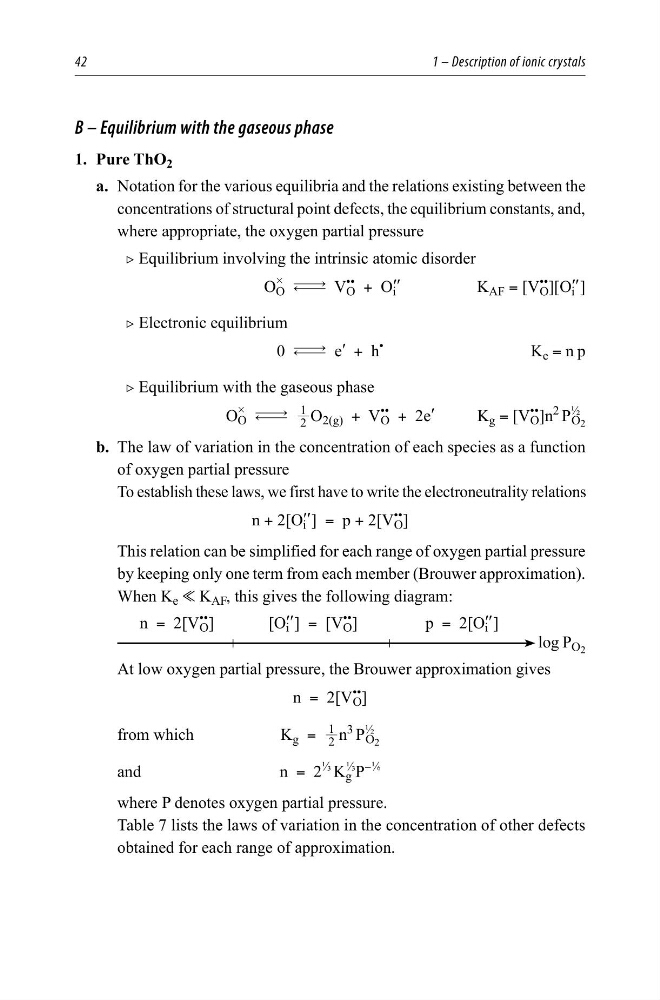
When K e % K AF , this gives the following diagram:
n = 2[V
••
O ]
[O ′′
i ] = [V
••
O ]
p = 2[O ′′
i ]
log P O 2
At low oxygen partial pressure, the Brouwer approximation gives
n = 2[V
••
O ]
from which
K g = 2
1
n
3
P
½
O 2
and
n = 2
⅓
K g
⅓
P
−¹⁄6
where P denotes oxygen partial pressure.
Table 7 lists the laws of variation in the concentration of other defects
obtained for each range of approximation.
1 – Description of ionic crystals
B – Equilibrium with the gaseous phase
1. Pure ThO 2
a. Notation for the various equilibria and the relations existing between the
concentrations of structural point defects, the equilibrium constants, and,
where appropriate, the oxygen partial pressure
2 Equilibrium involving the intrinsic atomic disorder
O
#
O m V
••
O + O ′′
i
K AF = [V
••
O ][O ′′
i ]
2 Electronic equilibrium
0 m e ′ + h
•
K e = n p
2 Equilibrium with the gaseous phase
O
#
O m 2
1
O 2(g) + V
••
O + 2e ′
K g = [V
••
O ]n
2
P
½
O 2
b. The law of variation in the concentration of each species as a function
of oxygen partial pressure
To establish these laws, we first have to write the electroneutrality relations
n + 2[O ′′
i ] = p + 2[V
••
O ]
This relation can be simplified for each range of oxygen partial pressure
by keeping only one term from each member (Brouwer approximation).
When K e % K AF , this gives the following diagram:
n = 2[V
••
O ]
[O ′′
i ] = [V
••
O ]
p = 2[O ′′
i ]
log P O 2
At low oxygen partial pressure, the Brouwer approximation gives
n = 2[V
••
O ]
from which
K g = 2
1
n
3
P
½
O 2
and
n = 2
⅓
K g
⅓
P
−¹⁄6
where P denotes oxygen partial pressure.
Table 7 lists the laws of variation in the concentration of other defects
obtained for each range of approximation.